Fan Curve vs System Curve: How to Find the Real Operating Point (With Example)

Executive Overview

In HVAC engineering, the fan does not operate at the airflow printed on the schedule merely because a designer wrote that number on a drawing. Nor does it operate at the duty point shown in isolation on a manufacturer’s submittal. The actual operating condition is established only where the fan curve intersects the system curve. That intersection determines the real operating point: actual airflow, actual static pressure, actual brake power, actual motor loading, and ultimately whether the installation will meet comfort, ventilation, smoke control, process, or energy objectives.

Try AI Integrated Cooling Load Calculator

This subject is fundamental, yet it is still one of the most misunderstood areas in building services engineering. Many projects experience under-delivery of airflow, unstable control, excessive noise, overloaded motors, or wasted energy because the operating point was assumed rather than engineered. In practice, that failure typically comes from one or more of the following:

FREE - Download Detailed Report (PDF)

• fan selection based only on nominal duty point without checking full fan curve behavior

• underestimation of system resistance

• failure to account for filter fouling, dirty coils, fire dampers, balancing dampers, sound attenuators, and terminal devices

• neglect of system effect and non-ideal inlet/outlet conditions

• misunderstanding of how variable air volume systems shift the system curve

• poor coordination between design intent, equipment selection, and field installation

For HVAC consultants, contractors, and technical decision-makers, understanding the relationship between fan curve and system curve is not just an academic exercise. It directly influences equipment sizing, CAPEX, energy consumption, controllability, commissioning success, tenant comfort, acoustics, and long-term operating cost.

At a consulting-grade level, the engineer must do more than plot two lines. The engineer must interpret what the intersection means in the real building. Is the selected fan stable at part load? Is the duty point near peak efficiency? What happens when filters load up? What happens after tenant fit-out introduces additional duct resistance? Will the motor still be within nameplate current? Is there sufficient static reserve for future variation? Are the control sequences aligned with the aerodynamic behavior of the fan?

The objective of this article is to explain, in a rigorous and practical way, how to determine the real operating point using fan curve and system curve analysis, how to validate it through calculation and engineering judgement, and how to use that understanding to make better design and commercial decisions. (Fan Curve vs System Curve)

Read related topics :

• Duct Static Pressure Calculation & Fan Selection Guide

• Most Common Mistakes in Jet Fan Ventilation System Design and Installation

• Ducted vs Jet Fan Ventilation Systems for Basement Car Parks

Why This Topic Matters in Real Buildings

The operating point governs whether the design actually works

In real buildings, the HVAC system succeeds or fails based on delivered performance, not design intent written on paper. A fan specified for 20,000 m³/h at 800 Pa external static pressure will not necessarily deliver that airflow once connected to actual ductwork, filters, coils, terminal devices, fire dampers, and control dampers. The building only receives the airflow associated with the actual intersection of the fan performance curve and the system resistance curve.

This matters because the consequences of a wrong operating point are rarely isolated to airflow alone. A 10–15% airflow shortfall can drive a chain reaction:

• insufficient cooling coil airside heat transfer

• increased space temperature deviation

• poor ventilation rates

• poor pressurization control

• unstable VAV performance

• inability to achieve smoke extract or stair pressurization objectives

• increased noise as balancing dampers are forced into restrictive positions

• unnecessary motor power increase if the fan drifts rightward into a high-flow region

Most fan problems are system problems

A common mistake in projects is to blame the fan manufacturer when a system fails performance testing. In many cases, the fan itself is not defective. The system resistance is simply higher than assumed, or the inlet/outlet arrangement creates adverse system effect, or the field-installed duct configuration deviates from the design model.

Examples seen regularly in projects include:

• abrupt elbows directly at fan inlet causing non-uniform velocity profile

• discharge transitions too short, generating additional dynamic losses

• flexible duct used excessively

• filters specified at clean condition only, without dirty allowance

• fire/smoke dampers not included properly in pressure calculations

• sound attenuator pressure drop ignored or underestimated

• tenant modifications increasing downstream resistance

• terminal devices selected late without pressure coordination

In such cases, the actual system curve rises above the design assumption, shifting the operating point leftward on the fan curve. The result is reduced airflow.

Read related topics :

• Why Your Fan is Consuming More Power Than Calculated

• Fan Pressure vs Airflow Explained

• Advanced Design of Basement Car Park Ventilation Systems

The topic has direct financial consequences

The difference between a correct and incorrect operating point affects both capital and operating expenditure.

If the engineer selects an oversized fan to “be safe,” the project may suffer from:

• higher equipment cost

• larger motor and starter/VFD size

• increased electrical infrastructure capacity

• excessive throttling losses

• poorer part-load efficiency

• higher noise and vibration risk

If the engineer undersizes or misjudges the system curve, the project may face:

• remedial ductwork modifications

• motor replacement

• impeller change

• VFD control issues

• claims and delays during testing and commissioning

• future occupant complaints and rework

For premium engineering clients, the value is not merely knowing the theory. The value lies in selecting the fan that delivers required performance with controllability, energy efficiency, resilience, and realistic field tolerance.

Core Engineering Principles

What is a fan curve?

A fan curve is a graphical representation of fan performance at a given fan speed, air density, and impeller geometry. It typically shows the relationship between:

• airflow rate, usually in m³/s or m³/h

• static pressure or total pressure, in Pa

• brake power, in kW

• efficiency, in %

• sometimes sound power level

For a fixed-speed centrifugal fan, as airflow increases, available static pressure generally decreases. The curve is not linear in a strict mathematical sense, though it is often approximated locally for engineering interpretation.

The fan curve is generated by test data under standardized conditions. It reflects the fan as tested, not automatically the fan as installed. Therefore, the engineer must apply correction and judgement where installation conditions deviate from the laboratory basis.

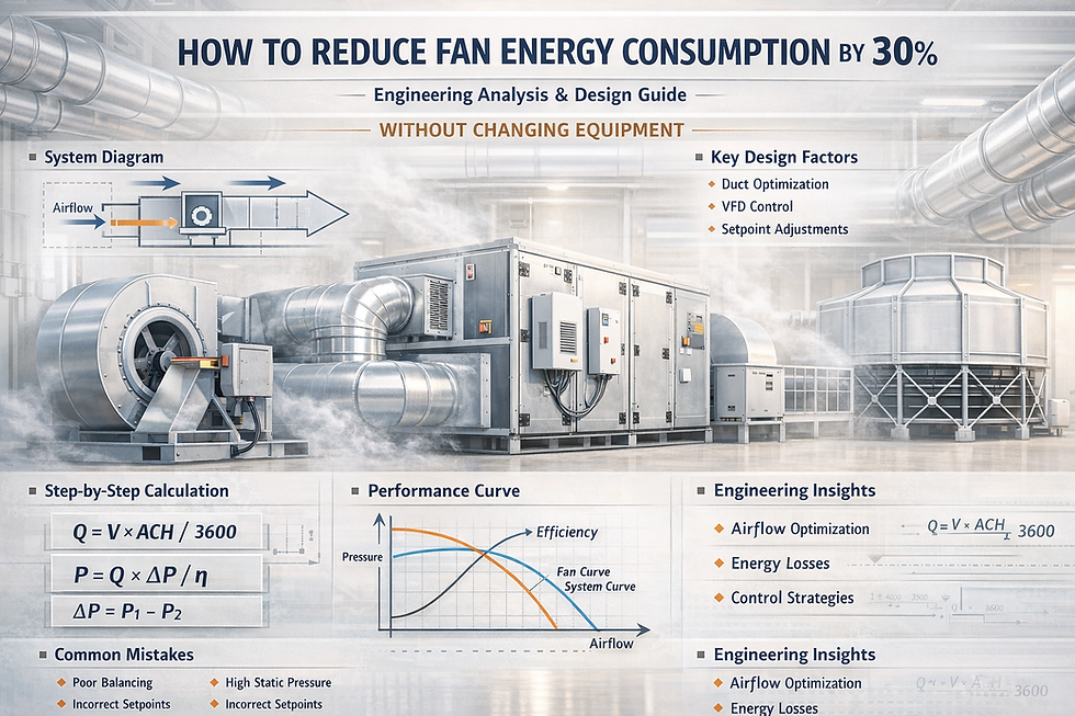
What is a system curve?

A system curve represents the pressure required by the air distribution system as a function of airflow. In most HVAC duct systems, pressure drop varies approximately with the square of airflow:

ΔP ∝ Q^2

So the system curve can be written as:

ΔP = KQ^2

Where:

• ΔP= system pressure loss, Pa

• Q = airflow rate, m³/s

• K = system resistance coefficient

If a known design point exists, the system constant can be derived from:

K = ΔPdesign / Q^2design

This quadratic relationship arises because most frictional and dynamic losses in ducts, fittings, coils, filters, and terminal devices scale roughly with velocity squared, and velocity is proportional to airflow for fixed area.

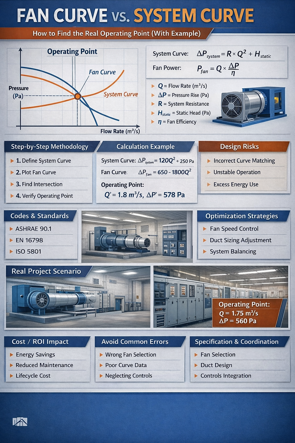
The real operating point

The real operating point occurs where:

Pfan(Q) = Psystem(Q)

That is the point at which the fan can generate exactly the pressure required by the system at that airflow. If the fan produces more pressure than the system requires at a given flow, the airflow rises. If it produces less, airflow falls. Equilibrium is reached only at the intersection.

This operating point determines:

• actual airflow delivered

• actual pressure developed

• actual shaft power

• actual motor load

• actual operating efficiency

Static pressure, total pressure, and why engineers confuse them

In practical HVAC fan selection, confusion often arises between:

• Static Pressure (SP)

• Velocity Pressure (VP)

• Total Pressure (TP)

The relation is:

TP=SP+VP

For many air handling and duct distribution applications, designers speak in terms of external static pressure because that is how AHUs and package units are commonly selected. However, fan manufacturers may provide total pressure curves or static pressure curves depending on fan type and test standard. The engineer must ensure that the pressure basis used for the system curve matches the pressure basis used for the fan curve.

Mixing external static pressure requirement with a fan total pressure curve without proper interpretation is a classic cause of selection error.

Fan laws

For geometrically similar operation and constant air density, the affinity laws are central:

Q ∝ N

P ∝ N^2

Power ∝ N^3

Where NNN is fan rotational speed.

These laws are essential for estimating how VFD control or speed adjustment shifts the fan curve. Reducing speed lowers airflow roughly linearly, reduces pressure roughly with the square, and reduces power roughly with the cube. This is why variable speed control is such a powerful energy optimization strategy.

Stable and unstable regions

Not all parts of a fan curve are equally desirable. Certain fans, especially forward-curved and some mixed-flow configurations, may exhibit unstable regions where small changes in system resistance produce erratic performance, surging, or non-repeatable operation. Engineers should avoid duty points near stall or unstable zones.

For premium-grade selection, the required operating point should usually sit:

• within a stable part of the fan curve

• reasonably near the best efficiency region

• with adequate margin for system variation

• without exceeding motor service factor or allowable sound criteria

Code, Standards, and Compliance Context

While fan curve and system curve analysis is an engineering performance issue rather than a code clause in isolation, it sits within a broader compliance framework.

AMCA standards

Fan performance selection and testing are heavily tied to AMCA standards. The most relevant references generally include:

• AMCA 210 for laboratory methods of testing fans for aerodynamic performance

• AMCA 300 for sound testing

• AMCA 201 for fans and systems

• AMCA certified ratings for validated published performance

From a consulting standpoint, it is prudent to specify fans with certified ratings so that the published fan curve is not merely a marketing representation but tied to recognized testing standards.

ASHRAE context

ASHRAE guidance is relevant for:

• duct design pressure calculations

• system effect considerations

• air distribution fundamentals

• energy efficiency expectations

• ventilation and comfort performance implications

ASHRAE handbooks, especially Fundamentals and HVAC Systems and Equipment, are commonly relied upon to interpret system resistance and application behavior.

SMACNA

SMACNA guidance is highly relevant for:

• duct friction design

• fitting loss coefficients

• recommended duct configurations

• inlet/outlet conditions

• system effect avoidance

• constructability details

Failure to respect good duct geometry often leads to a real system curve that is materially worse than the calculated one.

Energy codes and performance requirements

Energy regulations in many jurisdictions indirectly make operating point accuracy more important. If a fan operates away from its efficient region because it was poorly selected or because the system was poorly estimated, the building’s fan energy index, specific fan power, or overall energy performance can degrade.

Smoke control and life safety applications

In smoke extract, stair pressurization, and car park ventilation applications, operating point analysis becomes even more critical because the system resistance may vary significantly across modes, damper positions, and temperature conditions. For such systems, a single nominal operating point is often insufficient. Multiple-duty analysis is required.

Design Methodology Step by Step

Step 1: Define the required airflow properly (Fan Curve vs System Curve)

Begin with the required airflow based on the actual application:

• comfort cooling supply air

• outside air ventilation

• toilet exhaust

• kitchen exhaust

• smoke extract

• stair pressurization

• clean room process exhaust

The airflow must be derived from load, ventilation, pressurization, code, or process criteria. A fan selection cannot be credible if the airflow requirement itself is poorly defined.

Step 2: Build the system resistance model

Determine the total pressure loss through the full air path. This should include all major and minor losses:

• straight duct friction

• elbows, tees, branches, reducers, transitions

• coils

• filters, both clean and dirty

• fire dampers

• balancing dampers

• sound attenuators

• grilles, diffusers, louvers

• heat recovery devices where applicable

This is where many errors occur. The system curve is only as accurate as the pressure model behind it.

Step 3: Establish the design system point

Suppose the required design airflow is Qd​ and the total design pressure is ΔPd. Then the baseline system equation becomes:

ΔP = ΔPd(Q/Qd)^2

This is the simplest and most common way to construct the system curve from a known design point.

Step 4: Obtain the correct fan curve

Use manufacturer data at the intended fan speed and operating air density. Confirm whether the pressure basis is static or total. Obtain associated efficiency and power curves. Confirm certified performance where possible.

Step 5: Plot and find the intersection

Graphically or numerically find where the fan pressure equals the system pressure. This is the expected operating point.

Step 6: Check motor power and efficiency

At the operating point, determine:

• brake power

• fan efficiency

• motor size adequacy

• VFD suitability

• overload risk

A fan may technically intersect the system curve at the required airflow but still be a poor selection if it does so at low efficiency or near motor overload.

Step 7: Check off-design conditions

A premium selection always considers variation:

• dirty filters

• future system changes

• balancing condition

• minimum and maximum VAV operation

• seasonal density change if relevant

• smoke mode vs normal mode

• tenant fit-out allowance

Step 8: Review installation-induced system effect

Correct the system assumption if the inlet or discharge arrangement is poor. In real projects, system effect is often not a rounding error. It can materially shift the operating point.

Try AI Integrated Cooling Load Calculator

Step 9: Align controls with aerodynamic behavior

The fan, VFD, static pressure sensor location, and balancing strategy must be coordinated. A correct fan can still perform badly under a poor control sequence.

Step 10: Validate during commissioning

Final operating point is proven, not assumed. TAB and commissioning should verify:

• airflow

• static pressure

• motor current

• VFD speed

• damper positions

• terminal unit authority

• noise and vibration

Detailed Engineering Calculation Example

Consider a supply air fan for a medium-sized commercial office floor.

Design data

Required design airflow:

Qd = 18,000 m3/h

Convert to m³/s:

Qd = 18,000/3600 = 5.0 m3/s

Calculated total system static pressure at design airflow:

ΔPd = 900 Pa

This includes:

• ducts and fittings: 420 Pa

• cooling coil: 180 Pa

• clean filters: 120 Pa

• sound attenuator: 90 Pa

• fire damper and balancing allowance: 60 Pa

• terminal and diffuser allowance: 30 Pa

Total:

420+180+120+90+60+30=900 Pa

Construct the system curve

Using:

ΔP = KQ^2

K = 900/5.0^2 = 900/25 = 6

So:

ΔP = 36Q^2

where Q is in m³/s and ΔP in Pa.

Selected fan data

Suppose a candidate backward-curved centrifugal fan at chosen speed has approximate static pressure curve represented by:

Pfan = 1500−120Q

This is a simplified engineering approximation across the relevant range.

We find the operating point by equating fan pressure and system pressure:

1500−120Q = 36Q^2

Rearrange:

36Q^2 + 120Q - 1500 = 0

Divide by 12:

Q^2 + 10Q - 125 = 0

Use quadratic formula:

Positive solution:

Q = 30/6 = 5.0 m3/s

So the operating airflow is exactly:

Q = 5.0 m3/s = 18,000 m3/h

Pressure at this point:

ΔP= 36(5.0)^2 = 900 Pa

This is an exact match to design.

Fan power check

Assume fan total efficiency at this point is 72%.

Air power:

Pair = Q×ΔP = 5.0×900 = 4500 W

Shaft power:

Pshaft = Pair/η = 4500/0.72 = 6250 W

Pshaft = 6.25 kW

Assuming motor efficiency 92%:

Pinput = 6.25/0.92 = 6.79 kW

A motor size of 7.5 kW may be appropriate, subject to manufacturer data and service allowance.

What happens when filters load up?

Suppose dirty filter pressure adds an additional 100 Pa at design airflow, so revised system design pressure becomes:

ΔPdirty = 1000 Pa at 5.0 m3/s

New system constant:

Kdirty = 1000/25 = 40

New system curve:

ΔP = 40Q^2

Set equal to fan curve:

1500−120Q = 40Q^2

40Q^2 + 120Q −1500 = 0

Divide by 20:

That is about a 3.8% reduction. Depending on application, this may be acceptable or may require speed increase through VFD control.

What if system effect adds 150 Pa unexpectedly?

Suppose poor inlet arrangement and discharge condition effectively raise the design resistance to 1050 Pa at 5.0 m³/s.

New system constant:

K = 1050/25 = 42

System curve:

ΔP = 42Q^2

Set equal:

1500−120Q = 42Q^2

42Q^2+120Q−1500 = 0

Now the shortfall is about 5.6%. In a critical ventilation or cooling application, this can be operationally significant.

Engineering interpretation

This example illustrates an essential principle: a relatively modest increase in resistance can produce a meaningful airflow loss, especially if the fan curve is steep in the operating region. Therefore, good fan selection is not merely about matching one point. It is about understanding how robust the operating point is against system uncertainty.

Real Project Scenario

Consider a commercial retail development with a central AHU serving a high-occupancy tenant area. Design airflow was intended to be 28,000 m³/h. During commissioning, measured airflow was approximately 24,500 m³/h despite the fan operating near full speed.

Initial reaction on site was that the fan was undersized. However, detailed review showed the following:

• design pressure calculations had used clean filter pressure drop only

• sound attenuator submittal had a higher loss than basis of design

• a fire damper and access section arrangement created added turbulence

• discharge duct transition was shorter than recommended

• an additional branch balancing damper was almost closed because downstream duct balancing was poor

The combined effect raised actual system resistance materially above the design model. The original system curve used in fan selection was optimistic. The fan itself was performing close to its published curve.

Corrective strategy included:

• replacing the attenuator with a lower pressure drop model

• rebalancing branch resistances

• modifying discharge transition geometry

• revising control setpoints

• slightly increasing fan speed through VFD after current verification

The system eventually achieved acceptable performance without replacing the fan, but only after cost, delay, and coordination disruption. The lesson is straightforward: the “real operating point” is a project integration issue, not just a fan supplier issue.

Design Risks, Failure Modes, and Common Mistakes

Selecting from one duty point only

Many engineers or contractors select a fan because the catalog shows a nominal point close to required flow and pressure. This is not sufficient. The full curve must be reviewed to ensure:

• stable operation

• acceptable efficiency

• motor non-overload

• off-design resilience

Ignoring dirty conditions

Filters, coils, and heat recovery devices do not remain in their clean condition. Designs based only on clean pressure drops understate the system curve and create future airflow deficiency.

Confusing external static pressure with total fan pressure

This mistake can distort selection significantly. Pressure definitions must be aligned.

Neglecting system effect

System effect is routinely underestimated. Bad inlet approach or poor discharge arrangement can add significant effective resistance and alter performance.

Oversizing excessively for safety

Over-conservative fan oversizing often creates a different problem: the system is then throttled to achieve design airflow, wasting static pressure and energy. This is a poor engineering solution disguised as conservatism.

Operating too near stall or unstable region

Some fans can technically intersect the required system curve in a risky region. This can lead to noise, pulsation, unstable control, and unreliable operation.

Poor control sensor placement

In VAV systems, the static pressure sensor location matters. A badly placed sensor can drive the VFD to maintain the wrong pressure, forcing the fan into inefficient operation.

Underestimating future tenant changes

Shell-and-core or speculative commercial buildings often experience later fit-out changes that alter branch resistance. Reasonable reserve and controllability should be built into the selection.

Optimization Strategies

Select near the best efficiency region

The most robust fan selections are generally those where the operating point sits close to the best efficiency region while retaining controllable margin.

Use VFD control intelligently

Variable speed drives allow the fan curve to shift downward and leftward as required. This is powerful for:

• VAV systems

• part-load operation

• dirty filter compensation

• pressure reset control

When done properly, this reduces energy materially because of the cubic power relationship with speed.

Minimize system resistance before upsizing the fan

If a system cannot meet airflow, the first response should not always be “select a bigger fan.” Review the system. Lower-resistance filters, better duct geometry, smoother transitions, lower-pressure-drop attenuators, and better terminal coordination can often solve the problem more efficiently.

Avoid unnecessary throttling

Balancing should not rely on gross damper throttling caused by poor upstream design. Excessive artificial resistance wastes fan energy continuously.

Use static pressure reset

In VAV systems, static pressure reset reduces fan energy by allowing the setpoint to fall when demand is low. This prevents chronic over-pressurization of the duct system.

Try AI Integrated Cooling Load Calculator

Cost, Energy, and ROI Perspective

From a financial standpoint, fan operating point errors are highly significant because fan systems often run for long hours and because excess pressure translates directly into excess energy.

Suppose a fan is selected to operate at 5.0 m³/s and 900 Pa, with shaft power about 6.25 kW. If poor design forces operation at equivalent airflow using throttling and the effective required pressure rises to 1100 Pa, air power becomes:

Pair = 5.0×1100 = 5500 W

At the same 72% efficiency:

Pshaft = 5500/0.72 = 7.64 kW

Difference in shaft power:

7.64−6.25 = 1.39 kW

Assume annual operation of 4,000 hours:

Energy = 1.39×4000 = 5560 kWh/year

At electricity cost of 0.12 USD/kWh, annual extra cost is:

5560×0.12=667.2 USD/year

That may appear modest for one fan, but across multiple AHUs, stair pressurization fans, car park fans, smoke extract systems, and tenant units, the lifecycle penalty becomes substantial.

In large buildings, poor fan-system coordination can create tens of thousands of dollars in avoidable lifecycle cost, aside from comfort and commissioning impacts.

Advanced Engineering Insights

The shape of the fan curve matters

Two fans may both pass through the required duty point on paper, but their response to system variation may differ materially. A steeper fan curve can produce a more stable pressure-flow response in some systems. A flatter curve may react differently to resistance changes. Selection is not just about the duty point; it is about the curve shape relative to expected operating envelope.

System curve is not always a pure square-law curve

The square relationship is a useful and often accurate approximation, but real systems may include components with more complex behavior:

• control dampers with non-linear behavior

• VAV boxes changing geometry

• coils with face velocity-dependent effects

• louvers subject to wind influence

• parallel branches opening and closing

• smoke control modes with changing damper logic

For advanced projects, multiple system curves may need to be examined rather than a single idealized one.

Density effects should not be ignored in critical applications

At high altitude, high temperature, or smoke applications, air density changes affect performance. Engineers must ensure that manufacturer data and system requirements are interpreted on a consistent density basis.

Fan-system interaction affects acoustics

Operating away from the efficient region often correlates with higher turbulence, higher outlet velocity, and more noise generation. Therefore, accurate operating point analysis is also an acoustic control strategy.

Commissioning data can back-calculate the actual system curve

A strong commissioning engineer can use measured airflow and static pressure across several operating conditions to infer the actual system resistance and diagnose whether the issue lies with the fan, the system, or controls.

Specification and Coordination Considerations

Specifications should require:

• AMCA-certified fan performance where applicable

• complete fan curves with efficiency and power data

• motor selected for non-overload across operating range where required

• VFD compatibility

• submittal of sound data

• confirmation of operating point on submitted fan curve

• allowance for dirty filter condition where relevant

• clear identification of static vs total pressure basis

Coordination drawings should also address:

• adequate inlet straight length where practical

• proper discharge transitions

• access provisions for filter replacement without distortion of airflow path

• realistic routing that does not invalidate design friction calculations

• final device pressure coordination with architectural and fit-out design

A premium consultant will also ensure that control philosophy is included in the design narrative, because a well-selected fan without aligned controls still produces mediocre results.

FAQ (practical questions)

1. What is the real operating point of a fan?

It is the actual point where the fan performance curve intersects the system resistance curve. That point determines the real airflow and pressure in operation.

2. Why doesn’t a fan always deliver its scheduled airflow?

Because the fan only delivers the airflow that the connected system resistance allows. If the actual system resistance is higher than assumed, airflow will be lower.

3. Is the system curve always proportional to flow squared?

In most fixed-geometry HVAC duct systems, yes approximately. But real systems may deviate due to dampers, controls, variable geometry, and component-specific behavior.

4. What is the difference between fan static pressure and total pressure?

Total pressure equals static pressure plus velocity pressure. The engineer must match the system pressure basis with the manufacturer’s fan performance basis.

5. Why do dirty filters matter so much?

Dirty filters increase resistance, shifting the system curve upward and reducing airflow unless fan speed is increased or reserve pressure was planned.

6. Can balancing dampers solve poor fan selection?

Only partially. Excessive damper throttling wastes energy and may increase noise. It is not a substitute for correct fan-system design.

7. Should I always select a larger fan for safety?

No. Excessive oversizing can cause inefficiency, control problems, higher sound levels, and unnecessary capital cost. Better engineering is to estimate system resistance more accurately.

8. How does a VFD affect the fan curve?

Changing speed shifts the fan curve according to fan laws. Lower speed reduces flow, pressure, and power. This allows dynamic matching to system demand.

9. What is system effect?

System effect is the performance penalty caused by poor inlet or discharge conditions such as abrupt elbows, short transitions, or non-uniform airflow entering the fan.

10. How close should the duty point be to peak efficiency?

As a practical rule, it should be reasonably near the best efficiency region while still maintaining stability, controllability, and margin for system variation.

11. Why do some systems fail TAB even when the fan submittal looked correct?

Because the selection may have been based on an incomplete system pressure estimate, incorrect pressure basis, or ideal installation conditions that were not achieved on site.

12. Does the operating point affect motor current?

Yes. Motor current follows shaft power demand, which depends on actual airflow and pressure. A rightward shift on the curve can sometimes increase power significantly.

13. In VAV systems, do I still use one system curve?

Not really. VAV systems operate across a family of effective system curves depending on terminal positions and control logic. One design curve is only a reference point.

14. Is the cheapest fan usually the best commercial choice?

No. The cheapest first-cost fan can become the most expensive lifecycle choice if it operates inefficiently, fails commissioning, or requires remedial work.

15. What is the biggest practical mistake engineers make here?

Assuming the fan schedule duty point is the real operating condition without thoroughly validating the system curve, installation effect, and off-design behavior.

Conclusion

The relationship between fan curve and system curve is one of the most important practical concepts in HVAC engineering because it defines the difference between intended performance and actual performance. The real operating point is not a theoretical convenience. It is the condition at which the installed fan and the installed system reach equilibrium, and it governs airflow delivery, pressure, power, efficiency, acoustics, and reliability.

For serious MEP practice, it is not enough to select a fan at a nominal duty point. The engineer must construct the system curve honestly, interpret the fan curve correctly, confirm pressure basis, evaluate dirty and off-design conditions, account for system effect, coordinate controls, and verify operation in the field. This is where technical design becomes commercial value.

A well-engineered operating point delivers more than airflow. It delivers commissioning success, lower energy consumption, reduced lifecycle cost, fewer contractor disputes, better tenant outcomes, and stronger trust from clients. In premium engineering work, that is the difference between drafting a system and actually delivering one.

Author’s Note

This article is provided for guidance only. Final fan selection and system performance assessment should always be verified against project-specific design criteria, manufacturer-certified data, applicable codes, installation conditions, control strategy, and commissioning requirements. The engineering responsibility remains with the design and approval team for the specific project application.