AHU Mixing-Box Stratification: When Mixed-Air Sensors Mislead Diagnosis
Updated: 7 days ago
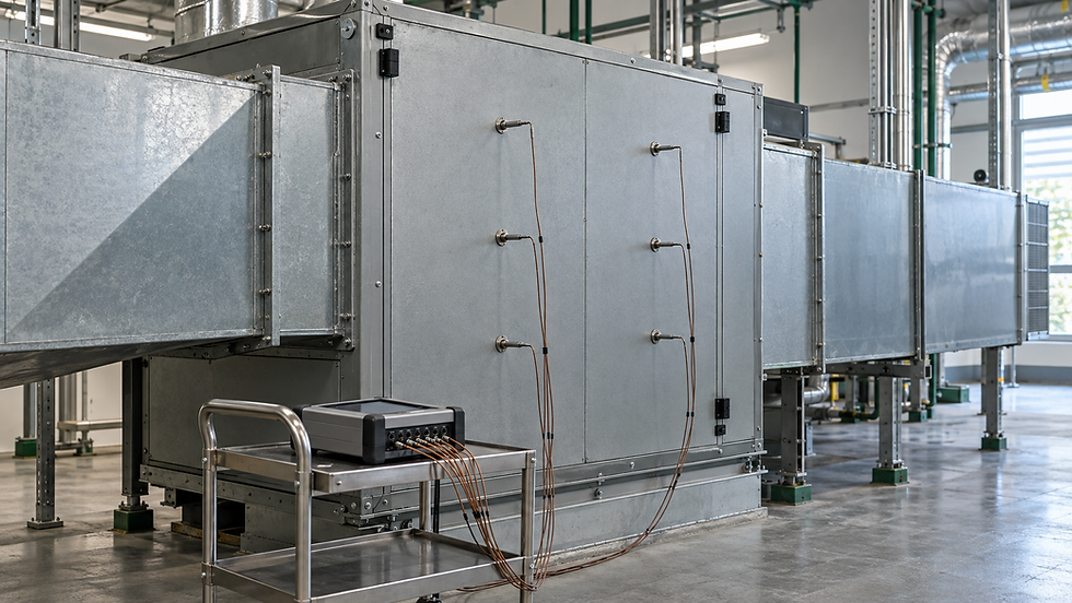
AI-generated editorial illustration; not a verified installation or construction detail.
A correct local reading can support the wrong conclusion
The BMS reports mixed air at 6°C while return air is 24°C and outdoor air is 0°C. A technician suspects that the outdoor-air damper is almost fully open. Another probe, lower in the same mixing section, reads 24°C. Either probe could be accurate at its own location.
Before replacing a sensor or changing the economizer sequence, determine whether the air streams are sufficiently mixed where temperature is measured. Nexora’s sensor and override diagnostic guide covers calibration and signal-path checks. This article develops the spatial problem: how a real temperature pattern can masquerade as a control fault.
Locate the air streams and the measurement plane
Outdoor and return air enter with different momentum, temperature and direction. A short mixing section can let those streams remain uneven across the downstream area. Damper position, fan flow and the relative inlet paths can change that pattern, so a sensor position that looked representative during one test may behave differently later.
Sketch the inlet openings, dampers, sensor locations and first downstream coil. Confirm whether a supposed mixed-air sensor is actually after a preheat coil or fan. Heat added between the inlet measurements and that sensor invalidates a simple mixing-only comparison. The separate AHU fan-heat article explains that thermal boundary.
Trane’s air-handler design guidance illustrates stratified outdoor and return streams and discusses engineered mixing and coil-protection options. It supports reviewing the whole arrangement, including available mixing distance. Installing a generic plate or baffle can add pressure loss, obstruct access or change coil-face velocity; any physical modification needs manufacturer and designer review.
Original example: three readings across one mixing plane
Consider a deliberately simplified steady winter case. Outdoor air is 0°C and return air is 24°C. Both have humidity ratio 0.0030 kg water/kg dry air, so their heat capacity per unit dry-air mass is equal. Ignore casing heat transfer, fan heat and condensation between the intakes and the measurement plane.
Total dry-air mass flow is 4.00 kg/s: 1.00 kg/s outdoor air and 3.00 kg/s return air. The bulk outdoor-air mass fraction is therefore 1.00 ÷ 4.00 = 25%. A fully mixed temperature would be 0.25 × 0 + 0.75 × 24 = 18°C.
Now divide the measurement plane into three equal-area bands with these assumed simultaneous observations: upper band 6°C carrying 0.80 kg/s; middle band 18°C carrying 1.60 kg/s; lower band 24°C carrying 1.60 kg/s. Unequal flow means that equal areas do not carry equal thermal weight.
The mass-weighted temperature is [(0.80 × 6) + (1.60 × 18) + (1.60 × 24)] ÷ 4.00 = 18°C. The simple arithmetic mean of the three temperatures is (6 + 18 + 24) ÷ 3 = 16°C.
The observations also close the inlet mass balance. At these common humidity conditions, the 6°C upper band contains 75% outdoor air, or 0.60 kg/s. The 18°C middle band contains 25%, or 0.40 kg/s. The 24°C lower band contains none. Total outdoor air remains 0.60 + 0.40 = 1.00 kg/s.
The 6°C sensor has not necessarily failed. It is reporting a cold-rich part of a stream whose bulk temperature is 18°C. Equally, the 24°C sensor cannot establish that the outdoor damper is closed. This is an illustrative pattern, not a prediction of which part of a real AHU will be coldest.
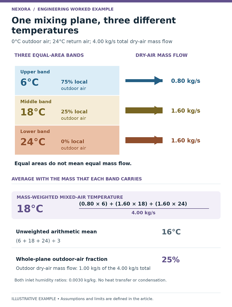
Original illustrative profile: [(0.80 × 6) + (1.60 × 18) + (1.60 × 24)] ÷ 4.00 = 18°C. Equal-area bands carry unequal dry-air mass flow. Both inlet streams have humidity ratio 0.0030 kg/kg; heat transfer and condensation are neglected. This is a measurement example, not a predicted installation profile.
Use temperature-derived outdoor fraction cautiously
For the example’s equal-heat-capacity assumptions, outdoor-air mass fraction = (return temperature − mixed temperature) ÷ (return temperature − outdoor temperature). Using 18°C gives (24 − 18) ÷ (24 − 0) = 25%. Substituting the upper-band 6°C gives 75%, while the lower-band 24°C gives 0%.
This inverse calculation requires a representative mixed condition, reliable inlet temperatures and no unaccounted heat or moisture process. Different humidity ratios require a proper moist-air energy and mass balance. Temperature-derived mass fraction also does not directly establish an outdoor volume flow without the relevant density and total-flow information.
Small inlet temperature differences make the calculation fragile even in well-mixed air. If return and outdoor temperatures differ by only 2 K, a 0.5 K mixed-sensor error alone changes the inferred fraction by 0.5 ÷ 2 = 25 percentage points, holding the inlet measurements exact. With a 24 K difference, the same error contributes about 2.1 percentage points.
Treat an inferred fraction outside 0–100% as a reason to investigate boundaries, sensor quality and timestamps. Do not simply clamp the result into range and retain it as proof of ventilation. Use an appropriate airflow measurement method for intake acceptance.
Test calibration and representativeness separately
First compare the installed probe with a suitable calibrated reference at the same location. Allow stabilization and consider both instruments’ uncertainty and response time. If they agree locally, applying an offset to match a distant point would conceal the spatial difference rather than correct calibration.
Next obtain a planned temperature map across the relevant plane using approved access points. Simultaneous measurements are preferable; a sequential traverse needs sufficiently steady conditions to separate changes over time from differences across space. Record outdoor and return temperatures, supply flow, damper positions and any active heating or cooling.
Retain individual temperatures, minimum, maximum and measurement locations. If estimating bulk temperature, obtain an appropriate airflow distribution and density basis as well. Multiplying every temperature by an equal weight is justified only when the represented mass flows are equal. A temperature map alone does not measure the airflow through each part of the plane.
Have qualified personnel arrange the test without entering operating equipment or exposing rotating machinery. Instrument installation may require isolation; operating measurements should use the equipment’s intended safe access arrangements.
Understand what an averaging sensor can and cannot show
Bravo Controls’ averaging-sensor description uses multiple sensing elements distributed across a mixing section. Such an arrangement can improve spatial coverage compared with a single point. Follow the selected device’s routing, support, bending and electrical requirements; a long probe bundled near one corner provides little representative coverage.
However, the output depends on the sensor’s actual averaging method and placement. An ordinary spatial average should not automatically be labelled a mass-weighted mean. In the original example, equal weighting produced 16°C although the mass-weighted value was 18°C. Nor does one averaged output reveal the lowest local temperature.
ASHRAE’s controls guidance notes that a satisfactory average mixed-air temperature can coexist with locally freezing air at a coil. It also distinguishes low-temperature detection used for protection. An averaging control sensor does not replace the specified protective device, its correct coverage or the approved freeze-protection sequence. The numerical example here stays above freezing and demonstrates measurement bias only.
A focused diagnostic closeout checklist
Confirm the physical identity and thermal boundary of each BMS temperature point.
Check the installed sensor against a co-located reference before changing calibration.
Map the temperature distribution at documented, stable operating conditions.
Preserve local extremes; apply mass weighting only with a defensible flow basis.
Repeat the relevant occupied low-flow and economizer conditions within the approved test plan.
Record whether the issue is sensor accuracy, point mapping, spatial representativeness or inadequate mixing, and obtain review of the proposed correction.
After an approved change, repeat the map and verify the intended control response. Do not close the issue merely because the dashboard now displays a plausible number. The useful outcome is a temperature signal that represents its control purpose, with local equipment protection independently maintained.
Related learning resource
Use Nexora’s HVAC Maintenance Checklist Pack to retain AHU temperature readings, defects and corrective-action records. Add the probe locations and operating conditions from the diagnostic test so future technicians can repeat a meaningful comparison rather than rely on an unexplained single temperature.
To extend this measurement-led approach across other AHU faults, explore the AHU Selection & Fault Diagnosis Handbook and preview. The reference includes 11 hypothetical troubleshooting cases, controls guidance and commissioning checklists. Get the complete handbook.
Sources and further reading
Engineering education only. Verify project conditions, applicable requirements and manufacturer data; use qualified professional judgment before design, selection, operation or maintenance decisions.


Comments