Pitot-Tube Duct Traverses: Convert Each Pressure Before Averaging

6 days ago

4 min read

Illustration of a pitot probe and blank pressure meter at a rectangular duct.

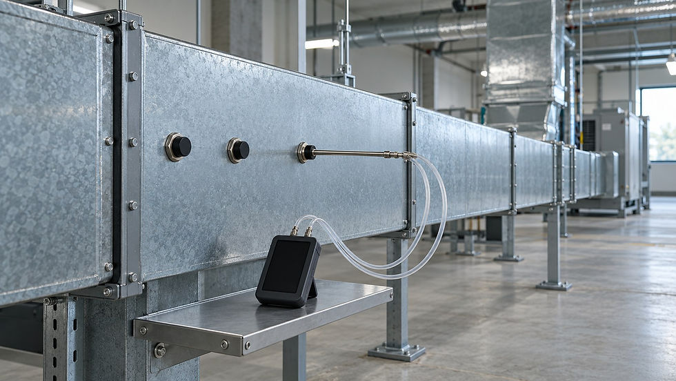
A spreadsheet can create airflow that was never measured

A duct traverse contains several velocity-pressure readings. A tempting spreadsheet shortcut averages those pressures, converts the average to velocity and multiplies by duct area. That sequence gives a different answer from converting each point first. In a nonuniform flow profile, the shortcut biases the result upward.

This article isolates that numerical error. It assumes a conventional Pitot-static tube, low-speed airflow, a common known density and properly obtained local velocity pressures. It does not make a poor traverse location acceptable or replace the project’s required testing and balancing procedure.

Preserve the order of operations

For the ideal unity-coefficient example, local velocity is v_i = √(2 × Δp_i / ρ), with velocity in m/s, velocity pressure in Pa and density in kg/m³. Apply the actual probe calibration coefficient and instrument corrections where required. Δp is total pressure minus static pressure at the measurement point; duct static pressure by itself is not the required input.

Calculate each local velocity, then combine the velocities using the traverse method’s area weighting. For equal-area cells represented by one point each, v_average = (v_1 + v_2 + … + v_n) / n. Flow is Q = A × v_average. TSI’s traverse application note explicitly warns against averaging Pitot pressures before converting them to velocity.

Worked example with four equal-area cells

Use a deliberately simplified four-cell illustration, not a recommended field point count. Assume an internal duct section of 1.00 m × 0.60 m, so total area is 0.60 m² and each cell represents 0.15 m². Air density is uniformly 1.20 kg/m³. The four velocity pressures are 2.4, 9.6, 21.6 and 38.4 Pa.

Point-by-point conversion gives √(2 × 2.4 / 1.20) = 2.0 m/s; the remaining velocities are 4.0, 6.0 and 8.0 m/s. Their equal-area mean is 5.0 m/s. Therefore Q = 0.60 × 5.0 = 3.00 m³/s, or 10,800 m³/h.

The shortcut first produces a mean pressure of 18.0 Pa. Converting that pressure gives √(2 × 18.0 / 1.20) = 5.477 m/s and a reported flow of 3.286 m³/s, approximately 11,831 m³/h. The apparent excess is 9.54%. Rounding cannot explain the difference; the two calculation sequences measure different quantities.

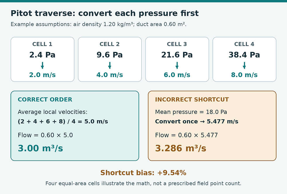
Four equal-area illustrative cells have pressures 2.4, 9.6, 21.6 and 38.4 Pa, converting to velocities 2, 4, 6 and 8 metres per second. Averaging velocities gives 3.00 cubic metres per second; averaging pressures first gives 3.286, a 9.54% upward bias.

Convert every local velocity pressure before area-weighted averaging. Four cells are used only to illustrate the numerical error.

Why the shortcut always runs high under these assumptions

At constant density, pressure is proportional to velocity squared. Taking the square root after averaging those pressures therefore returns the root-mean-square velocity: √[average(v²)]. The required equal-area average is the arithmetic mean of positive axial velocities. The root-mean-square value is at least as large, with equality only when all velocities match.

For the example, the mean square is (4 + 16 + 36 + 64) / 4 = 30, while the square of the mean is 25. The population variance is 5 (m/s)². Thus the shortcut-to-correct ratio is √(1 + 5/25) = 1.09545. Greater profile variation can make the error larger even if the instrument has excellent calibration.

This result explains the bias mathematically; it does not establish that every field discrepancy comes from averaging. Density errors, oblique flow, insufficient points and an unrepresentative measurement plane remain separate issues.

Keep cell weighting and air basis explicit

When measurement cells represent unequal areas, compute Q = Σ(A_i × v_i), using each cell’s assigned area. An unweighted mean is then inappropriate. Use the location and weighting rules of the adopted traverse procedure, particularly for circular ducts or nonuniform point spacing.

Use internal clear dimensions for the actual air passage and document lining or other geometry that changes the section. DwyerOmega’s velocity-measurement guidance discusses traverse points, probe alignment and density correction. Check whether an instrument reports actual or standard-air-equivalent flow before comparing its result with a schedule. A display labelled “velocity” does not reveal which averaging operation the instrument performs internally.

Build a calculation that can be audited

Keep a separate row for each point containing point identifier, represented area, raw pressure, density and converted velocity. Add the point flow contributions only after conversion. Retain raw pressure readings so another engineer can reproduce the result without relying on an instrument’s final aggregate.

For fluctuating readings, document the sampling period and averaging mode. The same nonlinear issue can arise within a time average at a point. Follow the instrument and test procedure rather than silently mixing instantaneous, pressure-averaged and velocity-averaged values.

Flag negative or near-zero differential pressures for investigation. Do not take absolute values or replace them with convenient positives to keep a square-root formula working. Check tube connections, zero drift, probe direction, measurement range and possible reverse or disturbed flow. An unsuitable Pitot measurement needs a suitable procedure, not a spreadsheet patch.

Finish with a repeatable field check

Select the best available traverse plane using the adopted method’s straight-run requirements and document nearby elbows, dampers or transitions. Check the instrument zero, tubing and calibration status, then repeat the traverse under stable system conditions. Correct arithmetic cannot compensate for a swirling profile that the probe cannot characterize.

The final report should include the point map, raw readings, conversion equation, density basis, area weighting and repeatability. That short chain of evidence makes a calculated airflow defensible and prevents an averaging shortcut from becoming a false balancing target.