AHU Filter Pressure Trends: Compare at a Common Airflow Before Calling the Filter Cleaner

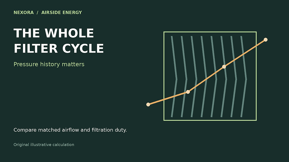
AI-generated illustrative scene, not a product screenshot or a completed-project photograph. The worked calculation below uses explicit example inputs.
An AHU filter differential-pressure trend falls from 100 Pa to 88 Pa after the building load reduces. It is tempting to report improved filter condition. But pressure loss changes with airflow as well as filter resistance. Without the matching airflow record, the direction of the pressure trend is not a reliable statement about cleanliness.
This example concerns an offline trend comparison. It does not set a replacement interval or alter a BMS alarm. Filters can require attention for reasons other than pressure loss, including damage, moisture, leakage or a manufacturer’s service requirement. Keep the approved maintenance and monitoring procedure in force while investigating a trend.
Use a measured curve rather than a universal exponent
Systemair’s filter-monitoring documentation associates calibration pressure with a reference airflow and describes recalculating an alarm limit at actual airflow. Alicat describes characterizing filters by recording pressure and flow together. These sources support the need for a pressure-flow relationship; they do not establish that every HVAC filter follows the same square law.
A local empirical model may be useful over a validated range. Write it as Δp = C × Q^n, where Q is the actual volumetric airflow through the filter, C represents the fitted resistance at stated conditions, and n is fitted from relevant data. The exponent and coefficient are model parameters, not universal material constants. A lookup table or manufacturer curve may be more appropriate.
Original example: the lower reading hides a higher comparison value
Assume an illustrative baseline curve for one installed filter bank has 100 Pa at 2.0 m³/s and 46.48 Pa at 1.2 m³/s. These hypothetical points correspond to n = 1.5. Assume the comparison stays within that airflow interval, uses the same air-density conditions and filter configuration, and that the later curve can be represented locally by the same exponent. The later reading is 88 Pa at 1.6 m³/s.
n = ln(100 / 46.4758) ÷ ln(2.0 / 1.2) ≈ 1.5
Later pressure normalized to 2.0 m³/s = 88 × (2.0 / 1.6)^1.5
Normalized pressure ≈ 123.0 Pa
Raw change = 88 − 100 = −12 Pa
Reference-flow change ≈ 123.0 − 100 = +23.0 Pa
Under the stated model, the raw reading fell 12% while the reference-flow comparison rose about 23%. That is a prompt to investigate increased resistance, not proof of a particular dust mass or remaining filter life. The values are invented to demonstrate the calculation; they are not performance measurements of a listed product.
An equivalent check compares the later reading with the baseline pressure expected at 1.6 m³/s. The baseline predicts 100 × (1.6/2.0)^1.5 = 71.55 Pa. The ratio 88/71.55 is about 1.230, matching the 23% increase. Keeping both versions in a worksheet makes a reversed airflow ratio easier to spot.

Local illustrative fit only; not a universal filter law or replacement threshold.
Test how much the assumed model matters
If n were 1.0, the same 88 Pa would normalize to 110 Pa; if n were 2.0, it would normalize to 137.5 Pa. This spread is not an uncertainty interval for the real filter. It shows why an unvalidated exponent can dominate the interpretation. Obtain the applicable curve or repeatable paired measurements before attaching a firm maintenance conclusion to the normalized value.
Avoid extrapolation toward zero flow: pressure signals approach instrument resolution, offsets become important and the normalized calculation can become unstable. Reject missing, negative or implausible airflow records. Do not use a fan-speed percentage as though it were measured filter airflow, especially if dampers, bypasses or fan arrangements change.
Preserve the measurement boundary
Record the pressure taps, transmitter range and zero check, filter identity, bank configuration, airflow method and timestamps. Confirm that both pressure ports span only the intended filter stage. A tubing problem or an extra component between the taps can mimic a resistance change. Keep original and normalized columns separate so the model never overwrites evidence.
The next useful deliverable is a graph containing the baseline curve, valid operating range and later paired observations, with excluded records explained. The AHU selection and fault-diagnosis handbook is a related review resource; this article does not claim that it implements this normalization or authorizes a new filter alarm.
Continue the calculation review
Sources and calculation basis
Primary references checked on 27 October 2026. The worked examples and diagrams are original illustrative calculations, not manufacturer selections or project approvals. Apply the stated limitations and the requirements governing the actual project.
Comments