Chiller IPLV vs Annual Plant Energy: Rebuild the Site Load-Bin Calculation
A lower chiller IPLV expressed in kW/TR can be useful when comparing equipment ratings, but multiplying that single number by annual cooling ton-hours does not establish a building’s annual plant electricity. The site may spend its operating hours at different loads and condenser conditions, and the plant meter may also include pumps, cooling towers and standby consumption.
A transparent first calculation is a site-specific load-bin model. Keep the cooling delivered, the operating hours and the corresponding electrical performance together in each bin. Then add the equipment included in the plant boundary. The example below is an invented scenario for checking the arithmetic, not a performance claim for a product or a forecast for a real building.
1. Read IPLV on its stated rating basis
ANSI/AHRI Standard 550/590-2023 defines part-load rating points at 100%, 75%, 50% and 25% load under specified conditions. In its kW/ton formulation, IPLV = 1 / (0.01/A + 0.42/B + 0.45/C + 0.12/D), where A through D are the respective point efficiencies in kW per refrigeration ton.
For an illustrative rating set of 0.62, 0.48, 0.42 and 0.46 kW/TR, that expression gives approximately 0.4498 kW/TR. The reciprocal form matters: simply taking an arithmetic weighted mean of those kW/TR values does not reproduce this rating. Use the stated standard edition and rating units when reviewing an actual submittal.
The rating conditions prescribe more than capacity fractions. The condenser conditions, water temperatures, flows and applicable rating procedures belong with the result. NPLV uses a nonstandard rating basis but remains a defined part-load metric; it does not automatically incorporate a site’s actual load chronology, staging or external auxiliaries. Neither label should be treated as an annual plant-meter reading.
2. Define the site model and electrical boundary
Assume a non-leap year with 8,760 hours and one nominal 500 TR water-cooled chiller. It operates for 4,000 hours and is off for 4,760 hours. All example cooling loads are met without cycling or unmet load. These assumptions simplify the arithmetic; an actual analysis must check the selected machine’s capacity and operating map at every relevant condition.
Hold leaving chilled-water temperature at an assumed 6°C. For the four operating bins, assume entering condenser-water temperatures of 30, 29, 28 and 27°C as load decreases. These are site-scenario inputs, not standard rating temperatures or suggested control setpoints. The example point efficiencies below are assumed to apply at those conditions and the scenario’s specified flows.
The electrical boundary includes the chiller package, chilled-water pumps, condenser-water pumps, cooling-tower fans and stated plant standby loads. It excludes building air-handler fans and terminal equipment. Before using real selection data, check whether package-integrated pumps or other devices are already included in chiller input power so they are not counted again.
3. Calculate each operating bin explicitly
For a bin with constant representative cooling load Q in TR, efficiency e in kW/TR and duration h in hours, chiller energy is Q × e × h in kWh. Here TR means a refrigeration ton, approximately 3.517 kW of cooling. Cooling ton-hours describe thermal service; electrical kWh describe the input used to provide it.
High-load bin: 500 TR for 200 h at an assumed 0.70 kW/TR gives 350 kW and 70,000 kWh. Cooling delivered is 100,000 TR·h.
Upper-middle bin: 375 TR for 800 h at 0.60 kW/TR gives 225 kW and 180,000 kWh. Cooling delivered is 300,000 TR·h.
Lower-middle bin: 250 TR for 1,600 h at 0.56 kW/TR gives 140 kW and 224,000 kWh. Cooling delivered is 400,000 TR·h.
Low-load bin: 125 TR for 1,400 h at 0.65 kW/TR gives 81.25 kW and 113,750 kWh. Cooling delivered is 175,000 TR·h.
The operating bins total 975,000 TR·h and 587,750 kWh of chiller electricity. Their energy-to-cooling ratio is approximately 0.6028 kW/TR. This is the scenario’s annual chiller input divided by delivered cooling, not a recalculated IPLV. It incorporates the assumed site hours and point performance rather than the standard rating weights.
For comparison, multiplying 975,000 TR·h by the unrounded illustrative rating, 0.449756 kW/TR, gives about 438,512 kWh. That shortcut is roughly 149,238 kWh below this scenario’s chiller total. The discrepancy follows from the different assumptions; it does not establish a general correction factor between IPLV and annual consumption.
4. Add auxiliaries and off-hour energy once
Assume combined external pump and tower-fan inputs of 70, 58, 44 and 35 kW in the four respective bins. Multiplying by their hours gives 14,000, 46,400, 70,400 and 49,000 kWh, for 179,800 kWh of operating auxiliaries. These are explicit illustrative inputs, not percentages automatically added to chiller power.

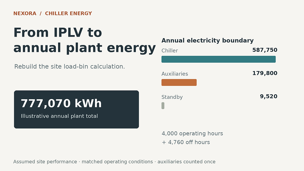
Original annual scenario: 4,000 operating hours plus 4,760 off hours. All efficiencies and auxiliary inputs are assumed; the total is not a manufacturer rating or a real-building forecast.
Also assume a total off-hour plant draw of 2 kW for the remaining 4,760 hours, giving 9,520 kWh. Count it only in the off-hour period because this example’s operating inputs already represent the equipment drawing power while the plant runs. Annual plant electricity is therefore 587,750 + 179,800 + 9,520 = 777,070 kWh.
Dividing by 975,000 TR·h gives approximately 0.7970 kW/TR on this annual energy boundary. The numerator includes standby while the denominator contains delivered cooling. That convention should be stated explicitly when comparing plants. A different meter boundary or omitted off-hour load can change the ratio without changing chiller performance.
5. Build bins that preserve the important relationships
Trane’s site-specific bin-analysis explanation describes why building loads, local weather and plant configuration matter beyond IPLV. For real projects, retain coincident load and weather data: separately sorting the warmest weather and highest loads can create operating combinations the building never experiences.
With multiple chillers, plant load fraction is not the same as each running chiller’s load fraction. A 50%-loaded plant with two equal machines can run one machine near full load or both near half load. Those cases need different machine inputs and possibly different auxiliary power. Represent the actual staging sequence, available capacity and load allocation.
Broad bins can conceal nonlinear performance. If condenser temperature, flow or chiller loading varies substantially inside a bin, subdivide it or calculate hourly energy. Avoid multiplying unrelated averages when load and efficiency are correlated. Include cycling, economizer operation, heat recovery and other modes only through supported data and a clearly defined allocation boundary.
6. Review the evidence behind the annual number
Obtain a complete annual schedule or document missing periods. Confirm operating and off-hour bins account for the intended year without overlap.
Match each performance point to load, chilled-water temperature, condenser conditions, flows and staging. Stay inside supported manufacturer data rather than extrapolating a favorable rating.
Reconcile pump, tower and package boundaries to avoid omissions and double counting. Compare modeled totals with suitable meter data when available.
Test uncertain hours and performance assumptions. Keep electricity cost and demand-charge analysis separate until the applicable tariff and coincident demand are established.
For wider plant-design context, the paid Chilled Water System Design Handbook is a related reference. The annual-energy decision should rest on the site calculation and its assumptions. A rating is a useful comparison input; a defensible plant forecast shows where every operating hour and electrical load entered the total.


Comments