Pump-Curve Interpolation: Stay Within the Selected Impeller Diameter and Catalog Points

Pump curves often arrive as crowded PDFs with several impeller diameters, efficiency contours and power lines on the same axes. A quick spreadsheet can accidentally combine points from different curves and still produce a plausible-looking answer. The most important interpolation check happens before the formula: confirm that both bounding points describe the same selected pump configuration.
The following worked example uses invented data to demonstrate a review method. It is not a catalog selection, a tested pump curve or permission to operate at the illustrated points. Its purpose is to make a small interpolation transparent, keep the calculation inside its data boundary and show what still needs manufacturer confirmation.
1. Lock the identity of the curve
Record the pump family and model, hydraulic size, impeller diameter, rotational speed, liquid and reference conditions, curve revision, and whether the data describe one pump or a combined arrangement. A frequency label alone may not establish actual shaft speed. If the equipment has been trimmed or modified, the original full-diameter plot may no longer represent it.
The Hydraulic Institute definitions tie pump performance to a particular model and speed and define best efficiency relative to speed and impeller diameter. That context matters when extracting a few numbers from a graphic. Every extracted point should retain the curve identity rather than becoming an anonymous flow–head pair.
Check the axis units as carefully as the equipment tag. Metres of liquid head, kilopascals, cubic metres per hour and litres per second are not interchangeable labels. Converting pressure to head requires the applicable liquid density. When digitizing a scan, verify both axes and any logarithmic scaling before reading coordinates.
2. Use two bounding points from the selected diameter
Assume an illustrative 180 mm impeller at 1,450 rpm has the following head points: 34 m at 10 m³/h, 31 m at 20 m³/h, 26 m at 30 m³/h, and 19 m at 40 m³/h. We want an approximate head at 26 m³/h. The bounding points are therefore 20 m³/h at 31 m and 30 m³/h at 26 m.
For a short linear segment, H = H₁ + (H₂ − H₁) × (Q − Q₁) / (Q₂ − Q₁). Substituting the example gives H = 31 + (26 − 31) × (26 − 20) / (30 − 20) = 28.0 m. The fraction 0.60 places the requested flow 60% of the way through that documented interval.
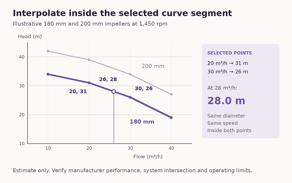
Invented data at 1,450 rpm. The highlighted segment uses only the 180 mm points. The separate 200 mm series must not supply a bounding point for this interpolation.
The result is an estimate along a straight chord between points. A real curve can have curvature within the interval, and reading a thick plotted line adds extraction uncertainty. Retain suitable precision: 28.0 m is more defensible here than 28.0000 m. For an actual selection, obtain the manufacturer’s selection output or higher-resolution data at the proposed conditions.
3. Show how a mixed-diameter error changes the answer
Now suppose the same illustrative chart also contains a 200 mm impeller, with 39 m at 20 m³/h and 34 m at 30 m³/h. If a reviewer mistakenly takes the 180 mm point at 20 m³/h, 31 m, and the 200 mm point at 30 m³/h, 34 m, the same interpolation formula returns 32.8 m at 26 m³/h.
The arithmetic is valid for the two entered coordinates, but the line describes neither impeller. It overstates the intended 180 mm estimate by 4.8 m, approximately 17.1%. A good worksheet should reject the calculation if the two records have different diameter, speed or model identifiers, even when their flows conveniently bracket the requested value.
Estimating an intermediate impeller diameter is a separate engineering task. It needs the manufacturer’s permitted trim range and a supported selection method, with updated performance checks. Do not treat the shortcut above as diameter interpolation. Likewise, scaling a curve with affinity relationships does not erase the assumptions or operating limits attached to the original data.
4. Keep interpolation separate from the operating point
An estimated head at a chosen flow does not establish that the installed system will operate there. Grundfos explains the duty point as the intersection of pump performance and system characteristics. A scheduled flow–head requirement and a predicted installed intersection serve different purposes and should be identified separately.
For an additional illustrative calculation, let the system characteristic be Hsystem = 8 + 0.030 Q², with head in metres and Q entered numerically in m³/h. The coefficient therefore carries units m/(m³/h)². The fixed 8 m is an assumed system requirement for this example, not building height automatically added to a closed recirculating loop.
Between 20 and 30 m³/h, the selected pump segment is Hpump = 41 − 0.50 Q. Equating the two produces 0.030 Q² + 0.50 Q − 33 = 0. The positive solution is approximately 25.86 m³/h at 28.07 m. It falls inside the same 20–30 m³/h segment, so the chosen segment is internally consistent with the calculation.
If the solution had fallen outside that interval, this local equation would no longer support it. Move to the appropriate documented segment and solve again. If no intersection exists inside the published applicable curve domain, flag the unresolved selection rather than extending the last line until it crosses the system curve.
5. Build hard limits into the worksheet
Store a configuration identifier with each point and require matching identifiers for interpolation. Sort points by flow and reject duplicate flow values that make the denominator zero.
Check that requested flow lies between both bounding flows and inside the manufacturer’s allowed operating region. A plotted endpoint alone does not establish every operating restriction.
Return an explicit out-of-range status outside the available data. Avoid spreadsheet options that extrapolate or silently clamp to the last point.
Preserve the source page, extraction date and method. Replace graphical estimates with manufacturer data when the selection approaches a limit or the uncertainty affects a decision.
6. Review the companion performance data
Head interpolation cannot establish efficiency, input power or suction suitability. Read their corresponding data at the same configuration and proposed duty, using the manufacturer’s definitions and applicable limits. Check the operating envelope and required suction margin with project-specific conditions; do not substitute a universal percentage of best-efficiency flow or a generic NPSH allowance.
Inferring field flow by reversing a head curve deserves particular care. On the illustrative 20–30 m³/h segment, a ±1 m head uncertainty corresponds to about ±2 m³/h before curve uncertainty, speed error or wear is considered. A flatter curve can turn a modest head error into a much larger flow ambiguity.
The paid Pump Head Calculator Design Suite v1.0 is a related resource for the system-head side of the review. Keep the manufacturer’s selected curve beside that calculation. A defensible result shows both the documented interpolation interval and the remaining selection checks.


Comments