MEP Labor Productivity: Separate Earned Hours from Hourly Cost

A cheaper hour does not prove better production
Two MEP crews can install the same accepted scope at the same hourly cost and still finish with very different labor totals. Conversely, a higher average hourly rate can accompany fewer hours and a lower installed cost. A weekly cost report becomes useful when it separates the quantity completed, hours consumed and cost per hour.
The operational question is specific: are remaining installation hours likely to match the estimate? Answer it with a consistent physical-progress measure before changing labor allowances. This workflow is a production-control calculation, not a method for assigning contractual responsibility for delays.
Define the unit and the hour before using a ratio
Construction productivity can be expressed as work-hours per installed unit. The Construction Industry Institute’s productivity-metrics presentation uses direct work-hours divided by installed quantity. The reciprocal, units per work-hour, is also useful, but its direction reverses: fewer hours per metre is better, while more metres per hour is better.
For a mixed installation package, define earned hours as accepted completed quantity multiplied by its agreed budget labor norm, summed across items. Earned hours are a baseline-weighted measure of output; they are not hours actually worked. Use labor-hours, not crew-hours: four people working eight hours consume 32 labor-hours.
In this article, productivity index PI = earned hours ÷ actual charged labor-hours for the same package. PI above 1 means fewer hours than the baseline; PI below 1 means more. Some organizations reverse this ratio, so print the equation beside the result rather than relying on the label alone.
The U.S. Department of Energy’s technical-analysis guide distinguishes standard-hour and actual-hour factors and warns that inclusion of idle time changes their meaning. Here the denominator includes all charged hours within the defined installation package, including its delays and rework. This deliberately avoids presenting a selected hands-on-work ratio as overall package performance.
Worked example: earned output and consumed hours
Assume a teaching package of 400 m of pipe installation at 0.80 labor-hour/m and 60 identical valves at 1.60 labor-hours each. The pipe norm includes its defined supports and joints; valve installation has a separate scope. Testing, insulation and general supervision are excluded from both the baseline and this package’s actual hours. These invented norms are not industry benchmarks.
The original budget is 400 × 0.80 + 60 × 1.60 = 416 labor-hours. At the reporting cutoff, inspection records confirm 100 m of complete pipe and 20 complete valves. Earned hours are 100 × 0.80 + 20 × 1.60 = 112 hours. Time records show 140 actual package hours.
Therefore PI = 112/140 = 0.80. Actual hours per earned hour equal 140/112 = 1.25. This means 25% more hours than the baseline for the accepted output. Calling it a “20% hours overrun” would confuse the index shortfall with the increase in hours required.
The completed work represents 112/416 = 26.9% of the baseline labor-weighted scope. Spending 140/416 = 33.7% of the budget hours is not evidence of 33.7% physical completion. Quantity acceptance and timesheet expenditure answer different questions.
Split the hourly-rate effect from the time effect
Use illustrative cost units, abbreviated CU, to keep the arithmetic independent of a country’s wage structure. Assume a budget loaded labor rate of 30 CU/hour and an actual average of 32 CU/hour. Both rates include the same cost categories. The earned output carries a budget labor value of 112 × 30 = 3,360 CU; its actual labor cost is 140 × 32 = 4,480 CU.
The 1,120 CU adverse difference separates exactly into two parts: extra-hours effect = (140 − 112) × 30 = 840 CU; hourly-rate effect = 140 × (32 − 30) = 280 CU. Their sum is 1,120 CU. This decomposition values excess hours at the budget rate and rate changes over all actual hours, so no interaction term is omitted.
If the same scope and cost boundary were used for earned-value cost control, its labor-only cost ratio would be 3,360/4,480 = 0.75. That is different from the hours index of 0.80. Do not label an hours ratio as the project’s overall cost performance index: materials, subcontract work and other costs are outside this example.
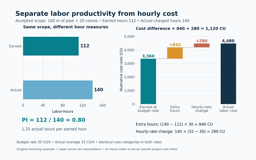
Original teaching example. Earned and actual hours share the same scope; CU means illustrative cost units.
Forecast remaining hours without pretending the past is destiny
The remaining baseline work is 416 − 112 = 304 earned hours. If the same work mix and observed PI of 0.80 continue, remaining actual hours are 304/0.80 = 380. Adding the 140 hours already spent gives a forecast of 520 hours, compared with the original 416.
Treat 520 hours as a conditional scenario. If upcoming areas have different diameters, connection methods, working heights or access restrictions, forecast those packages separately. If a verified coordination fix removes a recurring delay, show an alternative remaining-work assumption and track whether subsequent results support it. Changing the forecast is different from rewriting the original baseline.
Make the next weekly comparison credible
Freeze a common cutoff for quantities and timesheets. Define what counts as complete and use agreed milestones for partially finished assemblies. Keep damaged or rejected work from earning completion twice, while retaining the time spent repairing it. Separate approved added scope from original work and preserve the revision trail.
MCAA’s guidance on labor-productivity factors describes evaluating changed conditions before applying adjustment factors. An observed package PI does not by itself prove a particular cause. Check the actual constraints: late materials, workface access, repeated relocations, inspection waits, crew mix and drawing changes.
Close the loop with one measurable action and a later comparison on the same basis. For example, release complete valve-and-support kits to a defined work area, then compare its accepted quantities and charged hours with a comparable area. The goal is a better-supported remaining-hours estimate and a practical improvement in installation flow.
Sources and further reading
Continue your engineering workflow
The paid HVAC Estimation, BOQ and Job Costing Excel workbook brings rate libraries, BOQ build-ups, cost codes, actual costs and EAC reporting into one editable file. Use verified production inputs when building your forecast.



Comments