AHU Sensor Time Alignment: Separate Air-Transport Delay from Sensor Lag

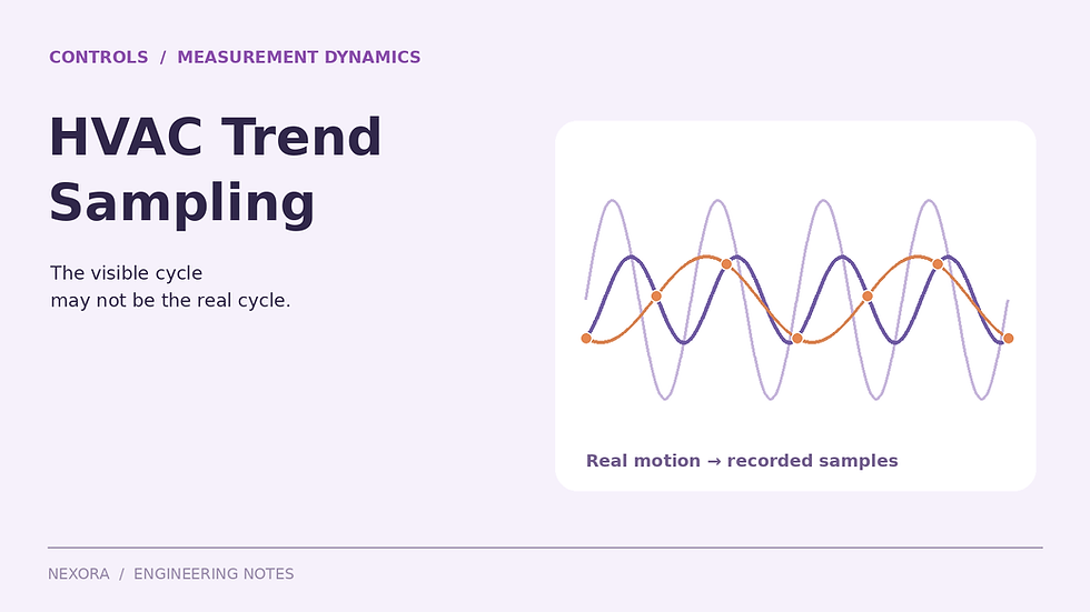
Original illustrative engineering schematic. The worked calculation below uses explicit example inputs.
A downstream supply-air sensor can report a warmer temperature than an upstream reference immediately after a cooling change even when the duct adds no heat. The changed air first has to travel to the downstream location. The sensor then needs time to approach the new temperature. Comparing equal timestamps without separating those effects can create a false heat-gain or slow-coil diagnosis.
There are at least three clocks to check: the physical travel of the air, the response of the sensing element and transmitter, and the way the control system timestamps and stores the reading. This article develops an original transport-plus-response example. It is a diagnostic interpretation method, not a proposal to retune a control loop from one trend plot.
Calculate the travel time on the actual air path
For a constant-area, unbranched duct with steady volumetric flow and approximately constant density, mean velocity is airflow divided by clear area. An ideal plug-flow travel time between two locations is length divided by velocity, or the intervening air volume divided by flow. Use clear internal area, not a dimension that includes insulation or lining.
Air speed v = Q/A.
Transport delay t_d = L/v = LA/Q.
For L = 36 m and A = 0.80 m², intervening volume V = 28.8 m³.
At Q = 4.0 m³/s: v = 5.0 m/s and t_d = 7.2 s.
At Q = 1.0 m³/s: v = 1.25 m/s and t_d = 28.8 s.
The fourfold reduction in airflow makes the ideal travel time four times longer. A single fixed timestamp shift cannot align both operating conditions correctly. For a route with several steady-flow sections, sum each section’s volume divided by its own flow. Branch takeoffs require the actual flow in each section, not the AHU total applied to the whole route.

For an illustrative 36 m air path, travel time is 7.2 s at 5 m/s or 28.8 s at 1.25 m/s. The separate 40 s first-order sensor time constant must not be confused with transport delay.
Add the sensor response separately
A first-order sensor model approaches a new air temperature exponentially. Its time constant τ is the time to complete about 63.2% of a step after the changed air reaches the sensing element. It is not a pure delay, and it is not the time to finish the response completely.
Manufacturer specifications can make the distinction concrete. Belimo’s 22DTM-51 data list separate response times for temperature and humidity, each at a stated duct airspeed. A combined probe therefore does not necessarily report both properties with matching dynamics. Use the exact instrument’s specifications, not a generic response time assigned to every point.
For this teaching example, assume the downstream temperature channel has τ = 40 s and the upstream reference resolves the imposed step essentially instantly. Keep τ the same at both flow rates solely to isolate transport effects. This is not a rating taken from the Belimo product; actual response can change with sensor construction, installation, airspeed and configured filtering.
For an upstream physical step from 20°C to 14°C at t = 0, the downstream indicated temperature is 20°C before t_d.
After arrival: T_indicated(t) = 14 + 6 exp[−(t − t_d)/40], with time in seconds.
Compare the two readings after one minute
At 4.0 m³/s and t = 60 s: T_indicated = 14 + 6 exp[−(60 − 7.2)/40] = 15.6028°C.
At 1.0 m³/s: T_indicated = 14 + 6 exp[−(60 − 28.8)/40] = 16.7504°C.
The low-flow sensor is about 1.15 K warmer at that instant, although both models have the same final air temperature and no duct heat gain. Its response started later. Assigning the whole difference to insulation failure, coil capacity or a bad calibration would misread a deliberately transient comparison.
For a first-order response, reaching 95% of the step takes −τ ln(0.05), approximately three time constants, after arrival. The total time measured from the upstream change is therefore about 127.0 s at high flow and 148.6 s at low flow in this example. Neither value is a universal commissioning waiting period.
NPL-associated research demonstrates that real air-temperature sensor response varies with sensor geometry and ventilation. That supports checking actual channel dynamics rather than importing a meteorological response recommendation as an HVAC acceptance rule. The test condition and the specific installed sensor both matter.
When flow changes during the journey, integrate displacement
The calculation V/Q uses constant flow over the parcel’s journey. During a rapid VAV change, neither the starting flow nor the ending flow alone describes that journey. For the same simplified constant-area duct, find the elapsed time over which accumulated volumetric displacement equals 28.8 m³.
Original changing-flow case: Q = 4.0 m³/s for the first 5 s after the upstream change, then 1.0 m³/s.
The first period displaces 20.0 m³.
The remaining 8.8 m³ takes 8.8 s, so arrival occurs at 13.8 s.
Using the initial flow throughout would predict 7.2 s; using the final flow throughout would predict 28.8 s. Both miss the 13.8 s result. In a sampled calculation, integrate Q over successive intervals until the required volume is reached, then interpolate within the last interval using an explicitly stated assumption for how flow varied.
This calculation follows an idealized transported signal, not every fluid particle in a turbulent duct. Dispersion, recirculation, branches and thermal interaction with duct surfaces spread and reshape a real temperature front. Use the volume calculation as a defensible first estimate and a check on fitted delays, not as proof of an exact physical arrival time.
A timestamp shift cannot remove response smoothing
Shifting a downstream trend backward by its transport delay can improve comparison with an upstream signal, but it does not undo the sensor’s exponential smoothing. If the upstream sensor is also slow, both response functions affect the observed difference. Simply adding their time constants as though they were two travel delays does not represent that comparison.
A more defensible check predicts each sensor’s output from a plausible physical signal, then compares predicted and observed trends. Avoid aggressively differentiating noisy readings to reconstruct the true temperature: inverse filtering can amplify noise and give a visually convincing but unsupported result. Preserve the raw trend beside every processed series.
Use a repeatable diagnostic sequence
Confirm point identity, sensor location, engineering units and whether timestamps represent acquisition, controller storage or server receipt.
Record the air path and clear volume between sensors, including branches and changes in section flow.
Collect airflow with the temperature trends so delay estimates follow the same operating history.
Obtain response-time and signal-filtering information for both channels; do not confuse display update rate with physical response.
Compare stable periods as well as transitions. A persistent stable temperature difference needs another explanation.
Document assumptions and uncertainty before using the aligned data to support a corrective action.
Sampling still matters, but it is a separate check. The trend-sampling review explains how a hunting loop can be misrepresented by a slow logging interval. The duct heat-gain review addresses a genuine steady temperature rise. Keeping those questions separate makes the diagnosis easier to defend.
Keep the supporting field evidence traceable with the Air Balancing Toolkit. Its workbook records airflow results, instrument calibration status and deficiencies, while its pocket handbook supports measurement practice. Retain the time-alignment model as a separate engineering record; the toolkit is not time-series analysis software.
Continue the calculation review
Sources and calculation basis
Primary references checked on 23 October 2026. The worked examples and diagrams are original illustrative calculations, not manufacturer selections or project approvals. Apply the stated limitations and the requirements governing the actual project.

Comments