HVAC Trend Sampling and Sensor Response Time: Avoid Aliasing a Hunting Control Loop
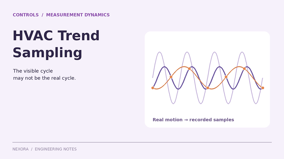
Before tuning a hunting HVAC loop, establish whether the trend can resolve the behavior you are diagnosing. The displayed curve has passed through a sensor, transmitter, controller input, communications path and historian. Each can change what reaches the screen. A smooth trace may conceal movement; an apparent slow cycle may be a sampling artifact. Preserve the existing settings while checking the evidence.
1. Map the measurement and logging chain
Record the sensor model and location, response-time specification, transmitter damping, controller scan time, point-update method and trend interval. Confirm whether the historian stores instantaneous values, interval averages or some other aggregation. Export raw timestamps and values; a graph’s connecting lines do not establish what happened between records.
Separate controller execution from trend capture. A controller might evaluate its input every second while the historian saves one point each minute. Faster logging also cannot refresh a network point that only updates every minute. Identify where each value originates and how old it can be when recorded. Include the setpoint, measured variable, output command, available actuator feedback and operating mode in the investigation.
2. Account for sensor response before interpreting amplitude
For an ideal first-order sensor with unity steady-state gain, use H(s) = 1/(1 + τs). The time constant τ is the time to complete about 63% of a step response. For a sinusoidal input at angular frequency ω, the amplitude ratio is 1/√[1 + (ωτ)²], and phase lag is arctan(ωτ). This follows the University of Michigan’s first-order system model.
Check which measured variable and test conditions a specification describes. For example, Vaisala’s HMD62/TMD62 specifications list humidity T63 as 15 seconds at 20°C, while temperature T63 under free convection is eight minutes. Those figures cannot be exchanged or assumed to represent a particular duct installation. Probe construction, airflow and configured filtering require verification.
3. Calculate how a real cycle becomes a misleading trace
Consider invented, steady-periodic test conditions: actual duct temperature T(t) = 16 + 2 sin(2πt/90) °C, with time t in seconds. Its period is 90 seconds and amplitude is 2 K. Assume a first-order sensor with τ = 30 seconds, no extra damping, negligible noise and instantaneous logging. This assumed time constant is unrelated to the manufacturer example above.
Angular frequency is ω = 2π/90 = 0.06981 rad/s. Therefore, ωτ = 2.0944.
The sensor amplitude ratio is 0.43087. Its output amplitude becomes 0.86174 K, with a peak-to-peak swing of 1.72348 K instead of the actual 4 K.
Phase lag is 64.48°, equivalent to 16.12 seconds at this particular frequency. This equivalent delay is frequency-dependent.
With a 60-second logging interval, the sample frequency is 1/60 Hz. The true frequency, 1/90 Hz, folds to |1/90 − 1/60| = 1/180 Hz: an apparent 180-second cycle.
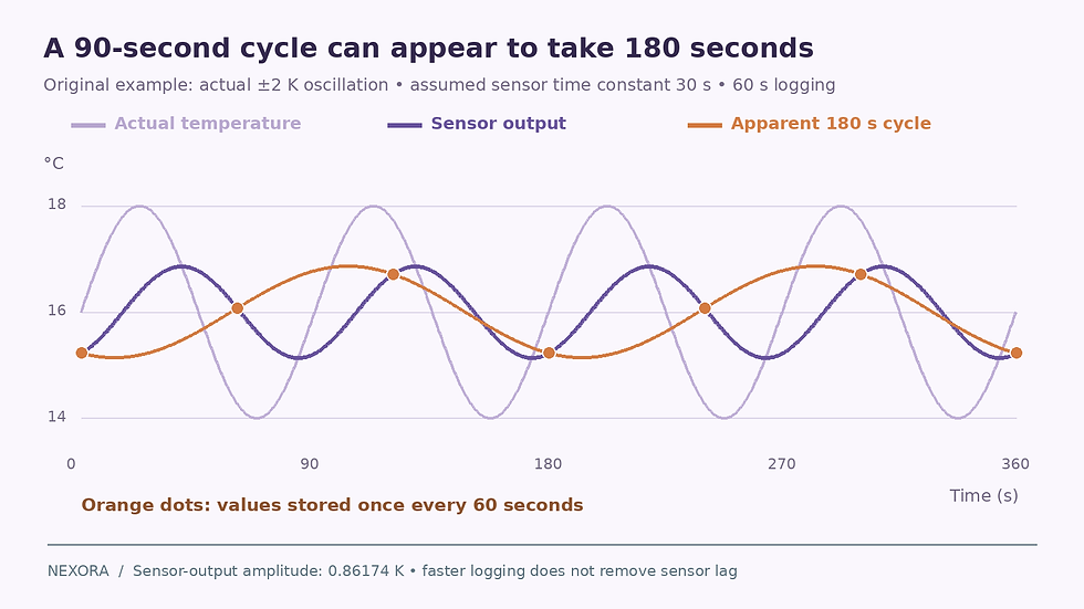
Original analytical example: a 30-second first-order sensor time constant reduces the 2 K input amplitude to 0.86174 K. One-minute samples are also consistent with a slower 180-second cycle.
For this chosen starting phase, the first four stored values are 15.222, 16.067, 16.710 and 15.222°C at 0, 60, 120 and 180 seconds. Logging every 90 seconds instead would repeatedly sample the same phase and produce a flat record. Both results can occur while the actual temperature continues oscillating.
4. Give the shortest relevant cycle enough samples
For a band-limited signal, the sampling rate must exceed twice its highest frequency to avoid aliasing. NIST’s discussion of digitizing pitfalls explains frequency folding and the role of filtering before sampling. The minimum theorem condition leaves little practical detail for diagnosing a loop’s waveform.
As a diagnostic starting point, aim for roughly 10–20 samples across the shortest cycle of interest, then verify that detail is sufficient. This is an engineering choice, not a universal BAS requirement. A six-second interval gives 15 samples per 90-second cycle here. It reveals the sensor output more clearly, but the calculated attenuation remains. Sensor lag alone is not proof of adequate anti-alias filtering.
5. Check change-of-value settings and timestamp meaning
Change-of-value logging records according to a change criterion rather than a regular clock interval. Johnson Controls’ trend documentation identifies separate COV-increment and periodic-sampling settings. Inspect the actual platform configuration, including any heartbeat or maximum interval. Small changes can remain unrecorded, and intervals between records can vary.
For the diagnostic capture, prefer regular time logging where supported. Retain event records for mode changes and alarms. When analyzing existing COV data, preserve the real event times; treating successive rows as equally spaced can invent timing. Interpolating them onto a regular grid does not recover missed extrema.
Verify clock synchronization, time zones and whether timestamps represent measurement, controller storage or server receipt. A 20-second relative offset equals 80° of phase at a 90-second period. That is enough to distort an apparent cause-and-effect sequence. Correct only offsets supported by evidence, and retain the originals. Do not shift curves until they merely look convincing.
6. Establish a defensible basis for tuning
Collect several complete cycles during a known operating mode, with unchanged setpoints and a reasonably stable load. Mark startups, overrides and transitions.
Compare commands with actual feedback where available. A valve command by itself does not establish stem movement or flow.
Check sensor placement and response against a suitable independent reference when practicable. Avoid treating numerical deconvolution of a noisy trend as proof of the true process.
Confirm available buffer capacity and system load before temporary high-rate logging. Preserve raw exports and document every capture setting.
Only then assess tuning, actuator behavior and sequence interactions. Change one authorized setting at a time, compare equivalent operating conditions and restore temporary logging afterward.
For broader air-balancing fieldwork, review the paid Air Balancing (TAB) Toolkit: Excel Workbook + Pocket Field Handbook.


Comments