Cooling Energy from Trend Logs: Weight Each Load by Its Time Interval

An exported cooling-load trend can look tidy while producing the wrong energy total. Three load values do not necessarily represent three equal slices of time. Logging interruptions, changes of value and different export settings can make the intervals unequal. The calculation must follow the timestamp and meaning of every observation, rather than the apparent spacing of rows in a report.
1. Confirm what each logged value means
A cooling load in kW is a rate of thermal energy transfer. Cooling energy in kWh is that rate accumulated over time. An interval-average load, an instantaneous sample and a cumulative energy register require different processing. Check the point description, logger configuration and meter documentation before choosing an equation.
ONICON's energy-meter overview describes thermal measurement using fluid flow and supply–return temperature difference. A derived trend may calculate load from these inputs, while a dedicated meter may also provide a cumulative energy register. Prefer comparing the trend integration with a valid register difference when both cover the same equipment and time boundary.
For water, an approximate instantaneous calculation is cooling kW = mass flow in kg/s × specific heat in kJ/(kg·K) × return-minus-supply temperature difference in K. Use appropriate fluid properties and consistent timestamps. Multiplying separately averaged flow and temperature difference can give a different answer from averaging their simultaneous product. This article assumes the load values have already been calculated correctly.
2. Integrate interval-average loads using actual duration
Consider an invented two-hour record with these explicitly defined interval averages: 100 kW from 08:00 to 08:15, 200 kW from 08:15 to 09:00, and 50 kW from 09:00 to 10:00. Each number represents the mean load over its entire named interval. The dataset is illustrative, not measured plant performance.
Convert each interval to hours and multiply it by the associated load. The first interval contributes 100 × 15/60 = 25 kWh. The second contributes 200 × 45/60 = 150 kWh. The third contributes 50 × 60/60 = 50 kWh. Their sum is 225 kWh of cooling energy over 2.00 hours.
The time-weighted average load is therefore 225/2 = 112.5 kW. The simple arithmetic mean of the three logged values is (100 + 200 + 50)/3 = 116.67 kW. Multiplying that unweighted mean by two hours gives 233.33 kWh, overstating this example by 8.33 kWh, or 3.70% of the correct total.
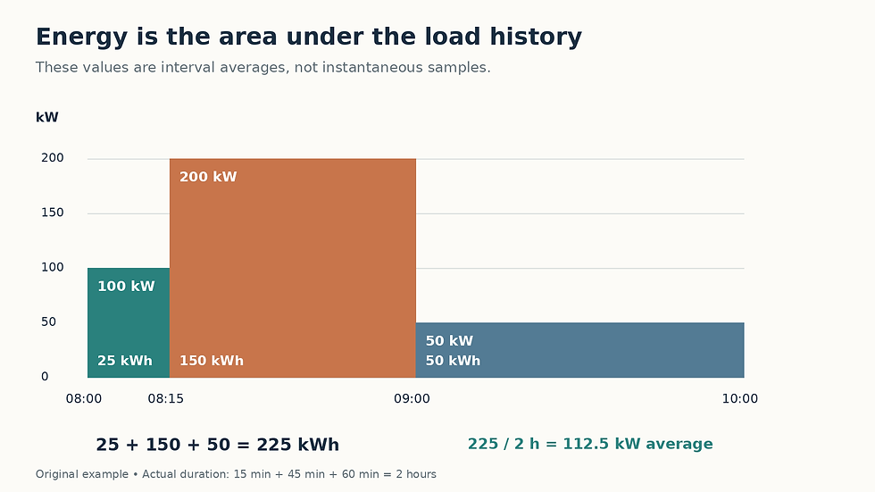
Original interval-average example. Block widths represent actual duration; the time-weighted average is 112.5 kW.
The error is not caused by rounding. The unweighted calculation gives the 15-minute first interval the same influence as the 60-minute third interval. A spreadsheet should carry separate columns for interval start, interval end, duration in hours, average load, interval energy and a validity flag. Summing interval energy makes the weighting visible and independently checkable.
3. Treat instantaneous samples as a different dataset
Suppose instead that 100, 200, 50 and 50 kW are instantaneous observations at 08:00, 08:15, 09:00 and 10:00. They do not establish the actual average between observations. If linear variation between adjacent samples is a reasonable approximation, trapezoidal integration estimates each interval as (starting kW + ending kW)/2 × duration in hours.
For these four point samples, the estimates are 150 × 0.25 = 37.5 kWh, 125 × 0.75 = 93.75 kWh and 50 × 1 = 50 kWh. The total is 181.25 kWh. This is not an alternative answer to the interval-average example: the two datasets assert different things about what happened between timestamps.
NumPy's trapezoidal integration documentation supports supplying explicit sample coordinates rather than assuming equal spacing, and notes that coordinates are processed in their supplied order. The same principle applies in a spreadsheet: sort timestamps intentionally, check duplicates and use each actual time difference. Convert time units explicitly so an integral in kW-minutes is not mislabeled kWh.
Trapezoids can be misleading across a known step change. If equipment switched from 100 to 200 kW at a documented event time, a linear ramp may invent load that never occurred. Split the interval at the event and use a justified piecewise representation. Conversely, holding a point reading constant until the next observation is an assumption unless the logger or operating evidence supports it.
4. Make missing time visible
An absent reading is not proof of zero cooling. Flag gaps before integrating and define a documented treatment appropriate to the analysis. Short interpolation may be defensible for a slowly varying process, but a long gap spanning plant startup or shutdown deserves separate investigation. Preserve estimated intervals as estimated, even when the completed chart looks smooth.
For example, suppose only 1.75 hours of the two-hour window have valid interval data and their known energy totals 200 kWh. Report 200 kWh over 1.75 valid hours with 87.5% time coverage. Its valid-time average is 114.29 kW. Dividing by the full two hours would produce 100 kW while silently assigning zero energy to the missing quarter hour.
If a reviewer approves a bounded estimate for the gap, show the assumed load, added energy and resulting uncertainty separately. Do not merge measured and filled records without a traceable flag. Likewise, do not carry the final sample forward beyond the reporting endpoint merely because the export has no following row.
5. Reconcile clocks, signs and registers
Use one time zone and resolve repeated or skipped local-clock times before computing durations. Check whether timestamps mark interval starts or ends.
Reject negative durations and investigate duplicate timestamps, overlapping exports and repeated rows.
Separate cooling and heating sign conventions. Do not replace all negative loads with positive values without understanding the meter definition.
Check cumulative-register resets, rollovers and unit changes before subtracting the first value from the last.
Compare only identical coverage windows and meter boundaries. Explain differences due to logging resolution, rounding and missing records.
Finally, label the result as thermal cooling energy. The 225 kWh example is not chiller input energy or a utility-bill saving. Estimating input requires matched performance and auxiliary-energy information. For broader hydronic-system context, see the Chilled Water System Design Handbook. Retain the original timestamps and calculation rows with the result so another engineer can reproduce the energy total without guessing how the logger worked.


Comments