Control-Valve Authority: Track the Changing Pressure Boundary
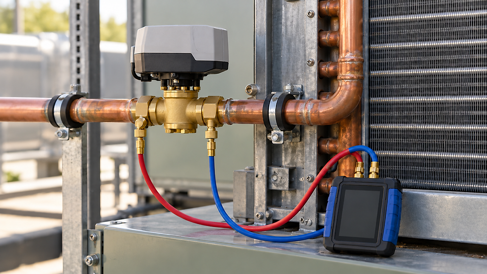
Put the pressure boundary on the schematic
A conventional two-way coil valve can pass design flow yet provide an awkward installed response. Reviewing its connection size or catalogue flow coefficient alone will not explain that behaviour. The pressure available across its branch, the other series resistances and the way that pressure changes during modulation must also be known.
Start by marking the two nodes that bound the controlled circuit. They might be local supply and return tees or the sensing points of a branch differential-pressure controller. List every component between those nodes. A valve-authority calculation based on that branch should not silently include unrelated plant losses or omit a balancing device inside the boundary.
State which authority definition is being used
At a stated design flow, define the simple resistance ratio a = Δpv,open/(Δpv,open + Δprest), where Δprest includes the coil, pipe and other series components inside the chosen boundary. Under an ideal constant branch differential pressure, this also equals the full-open valve pressure drop divided by the closed-valve differential pressure.
Valmet’s technical explanation describes authority using the operating valve drop and closed-valve differential, while noting that terminology is not internationally standardized. Declare the flow, valve position and pressure condition used in each numerator and denominator. Numbers calculated with different reference conditions should not be compared as though they were identical.
Belimo’s application guide explains that other components consume pressure when flow passes and that pump-head variation can add to the change seen by the valve. A variable-speed pump does not guarantee constant differential pressure at every coil branch; common distribution losses change as other branches modulate.
Worked example at a constant branch differential
Assume a water branch requires 2.00 L/s, equivalent to 7.20 m³/h. At that flow, the fully open control valve loses 20 kPa and the remaining branch loses 30 kPa. The design branch differential is 50 kPa and a = 20/50 = 0.40. With water relative density approximated as one, required Kvs is 7.20/√0.20 = 16.10 m³/h, using pressure drop in bar. Spirax Sarco’s water-valve sizing guide provides the flow-coefficient and authority framework.
For an original simplified model, let q = Q/Qdesign and y = Kv/Kvs. Assume steady incompressible flow, quadratic pressure losses, unchanged component geometry and no cavitation. At 50 kPa, the pressure balance is 50 = 20q²/y² + 30q². Rearranging gives q = y/√[0.40 + 0.60y²].
At y = 0.50, flow is 0.674 of design, or 1.348 L/s. At y = 0.25, flow is 0.378 of design, or 0.756 L/s. These are coefficient fractions, not actuator-stroke percentages. Converting them into travel requires the selected valve’s inherent characteristic. For a linear characteristic y approximately follows travel within its working range; an equal-percentage valve has a different mapping.
The model isolates why the installed relationship differs from the inherent constant-valve-pressure characteristic: closing the valve reduces branch flow, so the coil and pipe lose less pressure and leave more of the available differential across the valve. This is a hydraulic calculation of flow, not a prediction of cooling capacity or room-temperature response.
Now let the available differential rise
Suppose other branches close and the measured differential between the same two nodes rises from 50 to 80 kPa. Keep the example resistance coefficients unchanged. The new balance is 80 = 20q²/y² + 30q². At the same y = 0.50, flow becomes 0.853 of design, or 1.706 L/s, approximately 26.5% above the original 1.348 L/s.
At full opening, this simplified model predicts q = √(80/50) = 1.265, giving 2.530 L/s. The actual full-open valve and remaining-branch losses become 32 and 48 kPa, so their resistance ratio remains 32/80 = 0.40. Merely raising the available differential did not change the assumed valve-to-circuit resistance ratio.
However, the reference design valve drop divided by the new maximum branch differential is 20/80 = 0.25. That is a useful design-reference-to-maximum-pressure screening ratio, provided it is labelled as such. It must not be inserted into the original constant-boundary model as a replacement resistance ratio while simultaneously retaining the original design-flow normalization. That mixes two different conditions and produces the wrong flow prediction.
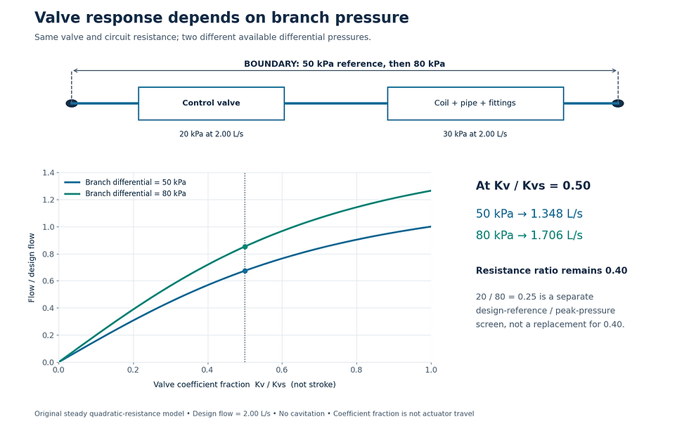
Original quadratic-resistance model. Horizontal axis is Kv/Kvs, not actuator stroke. Both curves retain the same valve-to-circuit resistance ratio; available branch pressure changes.
Choose a correction that addresses the observed cause
To achieve half the design flow, the same model needs y = 0.343 at 50 kPa but only y = 0.263 at 80 kPa. The pressure increase pushes the required coefficient lower. Whether this causes hunting depends on the actual valve characteristic, actuator resolution, linkage, controller tuning, sensor response and coil behaviour. A hydraulic ratio alone cannot establish the cause of unstable temperature control.
Check recorded branch differential and measured flow at several repeatable valve commands. Confirm the actuator reaches its commanded position, and separate stiction or a leaking seat from pressure-driven flow changes. Where excessive differential is verified, review pump reset and local differential-pressure control against the needs of all served branches. Do not reduce a central setpoint until the hydraulically demanding terminals are checked.
Keep control quality and pumping requirements together
A smaller Kvs increases the valve’s share of pressure loss at a specified flow, but also requires more pressure to deliver that flow. FlowCon’s authority discussion explains this control-versus-pumping trade-off. Use the project’s control requirements and selected-manufacturer data rather than treating one authority value as a universal mandatory target.
Document design and measured peak branch differential, design flow, open-valve drop, other branch losses, valve characteristic and the relevant control sequence. Check actuator close-off capability separately. If a pressure-independent valve is proposed, verify its own operating differential-pressure range and flow limits; this conventional pressure-dependent-valve model does not describe its internal regulating action.
Sources and further reading
Continue your engineering workflow
Connect valve decisions to pump duty, controls and commissioning with the Chilled Water System Design Handbook, a paid digital PDF containing worked calculations, valve schedules and a complete design example.


Comments