Estimating Chilled-Water Bypass Flow from Temperature Mixing

Temperature readings around a primary-secondary chilled-water bypass can help estimate how much water is short-circuiting between the supply and return. The calculation is especially useful when a permanent bypass flow meter is unavailable or a measured value needs an independent check. It requires a valid mixing arrangement, synchronized readings and at least one known flow to produce an answer in L/s.
Temperatures alone generally establish a ratio of flows. They do not establish the absolute flow rate. Treat the result as a diagnostic heat balance and verify it before changing chiller staging or protection settings.
1. Label four temperatures before opening the spreadsheet
Use these definitions consistently, including on the plant drawing:
Ts: common chiller supply temperature before the bypass supply junction.
Tr: building return temperature before the bypass return junction.
Tpr: mixed plant return temperature entering the operating chillers.
Tds: mixed distribution supply temperature leaving toward the building.
Qp: total operating primary flow; Qd: total distribution flow.
Define signed bypass flow Qb = Qp − Qd. Positive Qb means cold supply water flows toward the return junction. Negative Qb means warm return water flows toward the supply junction. Trane’s chilled-water training manual describes both excess and deficit flow and temperature-based mixing checks.
The following original examples assume steady operation, one uniform water composition, negligible heat gain between sensors and complete mixing before downstream measurement. Density and specific heat are treated as equal between streams. For materially different fluid properties, use a mass-and-enthalpy balance instead of the simplified volume-temperature equations.
2. Positive bypass flow: calculate the cold fraction entering the return
When Qp exceeds Qd, Qb = Qp − Qd flows from supply to return. At the return junction, Qp × Tpr = Qd × Tr + Qb × Ts. Rearranging gives Qb/Qp = (Tr − Tpr)/(Tr − Ts). The fraction is relative to primary flow, which matters when converting it into an absolute value.
Assume synchronized readings of Ts = 6.0°C, Tr = 12.0°C and Tpr = 10.2°C. An independently established primary flow is 50 L/s. The bypass fraction is (12.0 − 10.2)/(12.0 − 6.0) = 0.30. Therefore Qb = 15 L/s toward the return, and Qd = 50 − 15 = 35 L/s. In this ideal arrangement Tds equals Ts, or 6.0°C.
Check the thermal balance using water density 1 kg/L and specific heat 4.18 kJ/kg·K. The building-side load is 35 × 4.18 × (12 − 6) = 877.8 kW. The plant-side load is 50 × 4.18 × (10.2 − 6) = 877.8 kW. Agreement confirms the arithmetic for the stated assumptions; it does not independently validate the instruments.
An important reporting detail follows: the inferred bypass is 30% of primary flow but approximately 42.9% of distribution flow. A dashboard that says only “bypass percentage” is ambiguous. Always label the denominator.
3. Reverse bypass flow: calculate the warm fraction entering the supply
When Qd exceeds Qp, define the positive reverse-flow magnitude Qrev = Qd − Qp. Warm building return joins the chiller supply. The supply-junction balance is Qd × Tds = Qp × Ts + Qrev × Tr. Therefore Qrev/Qd = (Tds − Ts)/(Tr − Ts). This fraction is relative to distribution flow.
For a second, separate operating condition, assume Ts = 6.0°C, Tr = 12.0°C, Tds = 7.5°C and known distribution flow Qd = 60 L/s. The warm fraction is (7.5 − 6.0)/(12.0 − 6.0) = 0.25. Thus Qrev = 15 L/s, Qp = 45 L/s and the signed bypass flow is −15 L/s. The building receives 7.5°C water even though the chillers are delivering 6.0°C.
The thermal check is 60 × 4.18 × (12 − 7.5) = 1,128.6 kW on the building side, equal to 45 × 4.18 × (12 − 6) = 1,128.6 kW on the plant side. Under these assumptions Tpr equals Tr. A plant-supply sensor alone would miss the warmer water actually reaching the distribution system.
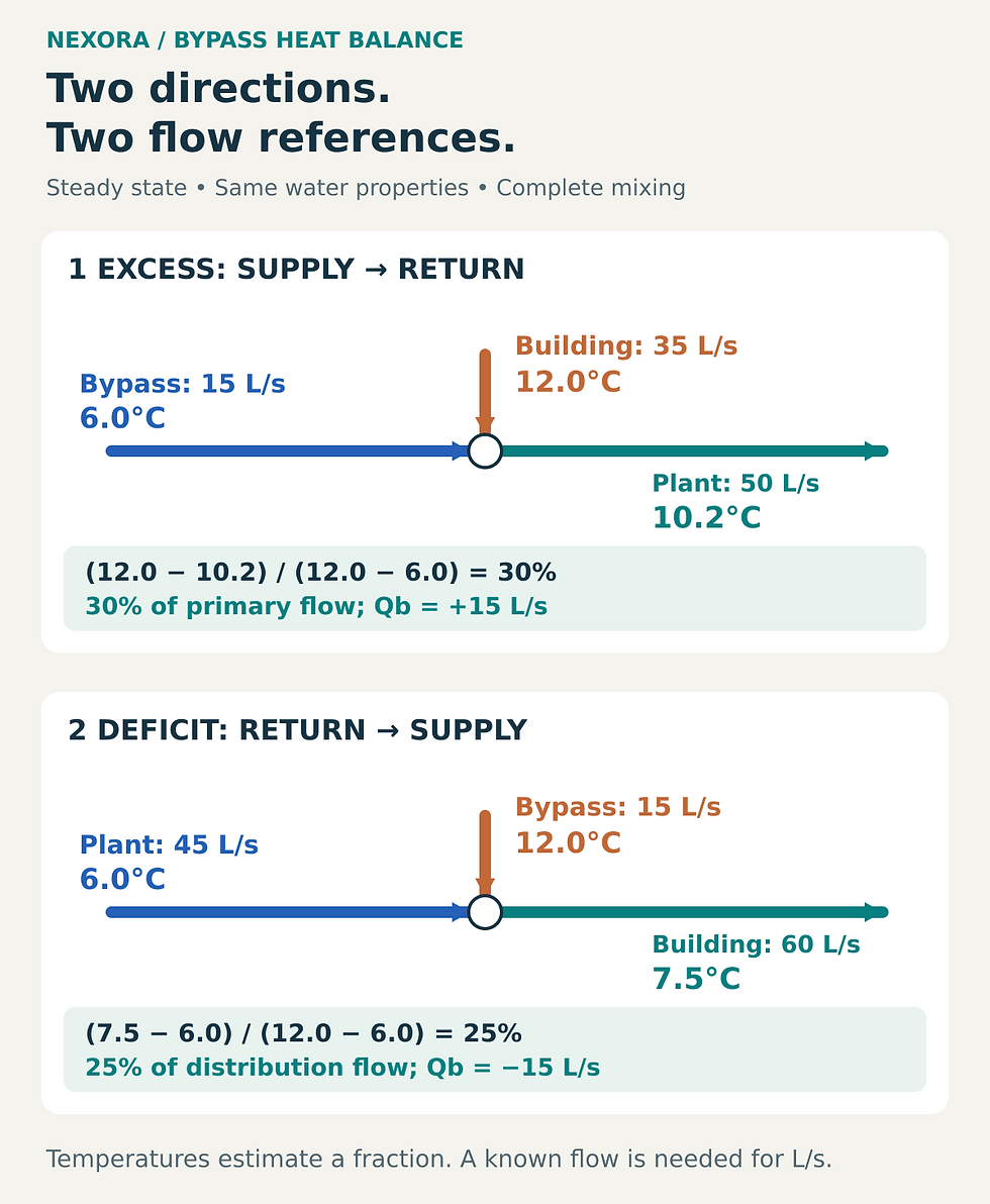
Original steady-state examples with uniform water properties and complete mixing. Positive bypass is supply to return; negative bypass is return to supply. Each percentage uses a different stated reference flow.
4. Test whether the temperature signal is large enough
In the positive-flow example, hold Ts and Tr fixed and vary only Tpr by ±0.2 K. At 10.0°C the inferred bypass fraction is 33.3%; at 10.4°C it is 26.7%. With primary flow fixed at 50 L/s, the estimate changes from 16.67 to 13.33 L/s. This is a single-sensor sensitivity test, not a complete uncertainty interval.
Uncertainty becomes more severe as Tr − Ts becomes small. Include all sensor uncertainties, their relative offsets, flow-meter uncertainty and timing errors in a proper assessment. Near zero bypass, small temperature differences may be insufficient to resolve direction confidently. Report an inconclusive result rather than forcing a precise signed value.
5. Recognize when the simple mixing model fails
Check sensor positions against the actual pipework. A sensor upstream of complete mixing can read one incoming stream disproportionately. A sensor far from the junction can include transport delay or heat gain. Temperature readings taken during pump or chiller transitions may describe different water parcels and cannot automatically be combined as a steady balance.
A large common connection can also permit simultaneous exchange in opposite directions. Trane’s discussion of chilled-water system decisions illustrates that mixing issue. A simple single-direction bypass model cannot reliably characterize such a condition. Additional measurements and a review of the physical arrangement are needed.
6. Turn the calculation into a field check
Confirm the hydraulic configuration and identify the operating chillers, pumps and alternative flow paths.
Mark the four temperature locations and verify which streams are actually mixed there.
Compare and check the installed sensors, then collect synchronized stable trends.
Calculate the appropriate flow fraction and state the independently known reference flow.
Compare against direct flow measurements where available and document uncertainty.
Ask the responsible controls and mechanical engineers to review discrepancies before changing sequences.
An impossible fraction, such as less than zero for the assumed direction or greater than one, is a reason to revisit the model and measurements. Do not silently clamp it into range. Protect all equipment flow limits while investigating.
For a more structured review of the wider plant, explore Nexora’s paid Chilled Water System Design Handbook. Keep this calculation alongside the actual schematic and trend record so the conclusion remains traceable.


Comments