Hydronic Ultrasonic Flow Sensors: Installation Checks Before Trusting Accuracy

An ultrasonic flow reading can look stable, repeatable and entirely believable while still being wrong enough to distort a chilled-water heat balance. The important question is not simply whether the display has settled. It is whether the installed measurement matches the conditions behind the meter specification.
For commissioning, divide the check into three boundaries: the water and pipe being measured, the ultrasonic instrument and its configuration, and the signal delivered to the building management system. A fault in any boundary can produce a convincing number. This article concerns transit-time instruments used with hydronic water or approved water/glycol mixtures.
1. Establish which type of ultrasonic meter is installed
An inline meter has a factory-defined measuring body. A clamp-on instrument sends ultrasound through the existing pipe wall, so installation data become part of the measurement. Do not transfer the setup assumptions of one type to the other. Siemens’ SITRANS FS220 catalog identifies pipe diameter, wall thickness and liquid viscosity among the customer-entered clamp-on parameters.
For a clamp-on survey, record the actual outside diameter, wall thickness, pipe material and any lining, then enter the fluid and temperature information required by that instrument. Nominal pipe size alone does not establish the water passage. If wall condition or an internal lining is uncertain, state that uncertainty rather than choosing a convenient library entry.
Record the model, sensor set, firmware, selected acoustic path and units. Retain a configuration export or photographs. These details make a later comparison meaningful, particularly if the same portable meter visits several pipe sizes during one shift.
2. Full pipe and a suitable velocity profile come first
Transit-time hydronic measurements need an appropriate, continuous acoustic path through the liquid. A location that traps air or drains partially can invalidate the reading. Siemens’ FSS200 installation instructions call for a location that remains full and, on horizontal pipe, a sensor plane that avoids gas or sediment blocking the path. Follow the selected sensor’s mounting and surface-preparation instructions.
There is no universal straight-run rule for every ultrasonic product. For example, Belimo’s 22PF-1..-1 technical data sheet specifies an inlet section of at least five nominal diameters for that family. That is a model-specific requirement, not permission to use five diameters for an unrelated clamp-on meter or every upstream disturbance.
Mark nearby elbows, tees, reducers, pumps and throttling valves on the survey sketch. Compare the actual arrangement with the manufacturer’s guidance for those disturbances. If the required location cannot be achieved, request an application review and document the limitation. A clean signal does not prove that a distorted velocity profile has become representative of the pipe average.
3. Worked check: a small bore error becomes a flow error
Consider an original sensitivity example with actual internal diameter D = 102 mm and actual flow Q = 8.40 L/s. Treat the cross-section as circular and assume the instrument has obtained the correct mean velocity. The area is π × 0.102²/4 = 0.008171 m², giving velocity v = 0.00840/0.008171 = 1.028 m/s.
If the flow calculation instead uses an internal diameter of 100 mm, while holding that velocity unchanged, it reports Qindicated = v × π × 0.100²/4 = 0.008074 m³/s, or 8.074 L/s. Equivalently, Qindicated/Qactual = (100/102)² = 0.9612. The result is approximately 3.88% low.
This is an area-only sensitivity calculation. A real clamp-on meter may also change its acoustic geometry and profile correction when pipe dimensions change, so 3.88% is not a complete error prediction or a correction factor to apply blindly. The calculation shows why checking the dimensional inputs is worthwhile before debating small flow discrepancies.
The same bias passes directly into a simplified heat balance when the other inputs remain fixed. With water density assumed to be 1 kg/L, specific heat 4.18 kJ/kg·K and temperature difference 5.0 K, the actual calculation is 8.40 × 4.18 × 5.0 = 175.56 kW. The area-biased reading gives 168.74 kW, a difference of 6.82 kW. These assumed properties are illustrative, not glycol values. For the wider diagnostic comparison, see Nexora’s airside–waterside cooling-coil heat-balance example.
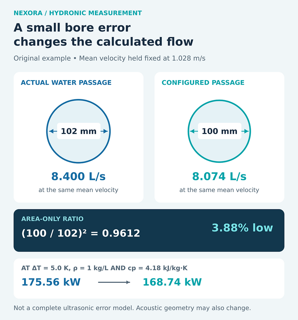
Original sensitivity example. Mean velocity is held fixed to isolate area error; real ultrasonic setup errors can also affect acoustic geometry and profile correction.
4. Read the accuracy statement at the operating flow
Check whether the specification is a percentage of reading, a percentage of full scale, a velocity-related term, or a combination. Also check the minimum usable flow, temperature range, fluid restrictions and any low-flow cutoff. A percentage without its denominator is not enough to assess suitability.
For illustration, ±1% of a 10 L/s full-scale range means ±0.10 L/s. At a measured 1.00 L/s that is ±10% of reading, whereas ±1% of reading would be ±0.01 L/s. These are invented comparison specifications, not claims about the products cited here. Resolution, repeatability and calibrated accuracy are separate characteristics.
Fluid composition matters twice when flow is used to calculate thermal duty: it can affect meter compensation, and it changes the density and specific heat used in the energy calculation. Caleffi’s hydronic field-measurement guidance discusses measuring flow and temperature together and selecting fluid properties for the operating condition. Record the verified glycol type and concentration rather than assuming that every blue or green liquid is equivalent.
5. Prove the complete measurement chain
Confirm that the measurement location remains full and satisfies the selected manufacturer’s installation requirements.
Check the configured pipe, liner and fluid data; inspect coupling and sensor spacing using the product procedure.
Record signal-quality diagnostics and investigate unstable or implausible results before averaging them.
Compare local and BMS readings at several safe, stable operating points. Check range, units, sign, pulse weight and analogue scaling.
Use an independent suitable reference where the acceptance requirement demands it, documenting both instruments’ uncertainties.
Retain the configuration, pipe sketch, operating conditions and limitations with the commissioning record.
Agreement between the display and BMS proves communication scaling, not hydraulic accuracy. A second meter installed on the same unsuitable location may repeat the same bias. Zero-flow checks are useful only when zero flow is independently established with a full pipe; stopping a pump does not exclude bypass or reverse flow. Do not interrupt critical circulation solely to create a convenient test condition.
The responsible commissioning or mechanical engineer should review installation exceptions and the uncertainty needed for balancing, energy reporting or equipment protection. Do not revise chiller minimum-flow limits on the strength of an unverified spot reading. For the wider system context, explore Nexora’s paid Chilled Water System Design Handbook.


Comments